About the Project

Visit (-- RXLARA.COM --) pharmacy buy Super P Force jelly over counter. Sildenafil Citrate Super P Force jelly Dapoxetine 160

AdvancedHelp

(0.017 seconds)

21—30 of 821 matching pages

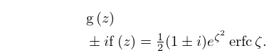
21: 7.5 Interrelations
7.5.6 e ± 1 2 π i z 2 ( g ( z ) ± i f ( z ) ) = 1 2 ( 1 ± i ) ( C ( z ) ± i S ( z ) ) .
7.5.7 ζ = 1 2 π ( 1 i ) z ,
7.5.8 C ( z ) ± i S ( z ) = 1 2 ( 1 ± i ) erf ζ .
7.5.9 C ( z ) ± i S ( z ) = 1 2 ( 1 ± i ) ( 1 e ± 1 2 π i z 2 w ( i ζ ) ) .
7.5.10 g ( z ) ± i f ( z ) = 1 2 ( 1 ± i ) e ζ 2 erfc ζ .
22: 32.10 Special Function Solutions
For example, if α = 1 2 ε , with ε = ± 1 , then the Riccati equation is … Solutions for other values of α are derived from w ( z ; ± 1 2 ) by application of the Bäcklund transformations (32.7.1) and (32.7.2). … with n , and ε 1 = ± 1 , ε 2 = ± 1 , independently. … with n and ε = ± 1 . In the case when n = 0 in (32.10.15), the Riccati equation is …
23: 12.2 Differential Equations
Standard solutions are U ( a , ± z ) , V ( a , ± z ) , U ¯ ( a , ± x ) (not complex conjugate), U ( a , ± i z ) for (12.2.2); W ( a , ± x ) for (12.2.3); D ν ( ± z ) for (12.2.4), where … The solutions W ( a , ± x ) are treated in §12.14. In , for j = 0 , 1 , 2 , 3 , U ( ( 1 ) j 1 a , ( i ) j 1 z ) and U ( ( 1 ) j a , ( i ) j z ) comprise a numerically satisfactory pair of solutions in the half-plane 1 4 ( 2 j 3 ) π ph z 1 4 ( 2 j + 1 ) π . …
§12.2(vi) Solution U ¯ ( a , x ) ; Modulus and Phase Functions
When z ( = x ) is real the solution U ¯ ( a , x ) is defined by …
24: 19.22 Quadratic Transformations
4 ( p ± 2 a 2 ) = ( p 2 x 2 ± p 2 y 2 ) 2 .
Again, we assume that a 0 g 0 (except in (19.22.10)), and define c n = a n 2 g n 2 . …
4 ( z ± 2 a 2 ) = ( z 2 x 2 ± z 2 y 2 ) 2 .
However, if x and y are complex conjugates and z and p are real, then the right-hand sides of all transformations in §§19.22(i) and 19.22(iii)—except (19.22.3) and (19.22.22)—are free of complex numbers and p ± 2 p 2 = ± | p 2 x 2 | 0 . … These relations need to be used with caution because y is negative when 0 < a < z + z ( z + 2 + z 2 ) 1 / 2 . …
25: 8.12 Uniform Asymptotic Expansions for Large Parameter
8.12.5 e ± π i a 2 i sin ( π a ) Q ( a , z e ± π i ) = ± 1 2 erfc ( ± i η a / 2 ) i T ( a , η ) ,
8.12.16 e ± π i a 2 i sin ( π a ) Q ( a , a e ± π i ) ± 1 2 i 2 π a k = 0 c k ( 0 ) ( a ) k , | ph a | π δ ,
8.12.18 Q ( a , z ) P ( a , z ) } z a 1 2 e z Γ ( a ) ( d ( ± χ ) k = 0 A k ( χ ) z k / 2 k = 1 B k ( χ ) z k / 2 ) ,
for z in | ph z | < 1 2 π , with ( z a ) 0 for P ( a , z ) and ( z a ) 0 for Q ( a , z ) . …
d ( ± χ ) = 1 2 π e χ 2 / 2 erfc ( ± χ / 2 ) ,
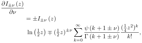
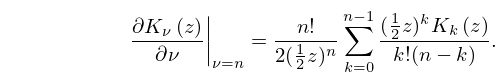
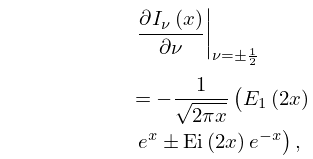
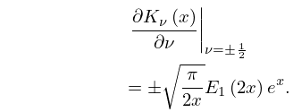
26: 10.38 Derivatives with Respect to Order
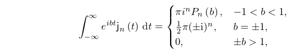
10.38.1 I ± ν ( z ) ν = ± I ± ν ( z ) ln ( 1 2 z ) ( 1 2 z ) ± ν k = 0 ψ ( k + 1 ± ν ) Γ ( k + 1 ± ν ) ( 1 4 z 2 ) k k ! ,
10.38.3 ( 1 ) n I ν ( z ) ν | ν = n = K n ( z ) + n ! 2 ( 1 2 z ) n k = 0 n 1 ( 1 ) k ( 1 2 z ) k I k ( z ) k ! ( n k ) ,
10.38.4 K ν ( z ) ν | ν = n = n ! 2 ( 1 2 z ) n k = 0 n 1 ( 1 2 z ) k K k ( z ) k ! ( n k ) .
10.38.6 I ν ( x ) ν | ν = ± 1 2 = 1 2 π x ( E 1 ( 2 x ) e x ± Ei ( 2 x ) e x ) ,
27: 10.59 Integrals
10.59.1 e i b t 𝗃 n ( t ) d t = { π i n P n ( b ) , 1 < b < 1 , 1 2 π ( ± i ) n , b = ± 1 , 0 , ± b > 1 ,
where P n is the Legendre polynomial (§18.3). …
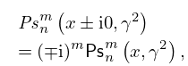
28: 30.6 Functions of Complex Argument
The solutions …of (30.2.1) with μ = m and λ = λ n m ( γ 2 ) are real when z ( 1 , ) , and their principal values (§4.2(i)) are obtained by analytic continuation to ( , 1 ] . … with A n ± m ( γ 2 ) as in (30.11.4). …
29: 4.25 Continued Fractions
4.25.1 tan z = z 1 z 2 3 z 2 5 z 2 7 , z ± 1 2 π , ± 3 2 π , .
4.25.2 tan ( a z ) = a tan z 1 + ( 1 a 2 ) tan 2 z 3 + ( 4 a 2 ) tan 2 z 5 + ( 9 a 2 ) tan 2 z 7 + , | z | < 1 2 π , a z ± 1 2 π , ± 3 2 π , .
4.25.3 arcsin z 1 z 2 = z 1 1 2 z 2 3 1 2 z 2 5 3 4 z 2 7 3 4 z 2 9 ,
4.25.4 arctan z = z 1 + z 2 3 + 4 z 2 5 + 9 z 2 7 + 16 z 2 9 + ,
4.25.5 e 2 a arctan ( 1 / z ) = 1 + 2 a z a + a 2 + 1 3 z + a 2 + 4 5 z + a 2 + 9 7 z + ,
30: 4.35 Identities
4.35.1 sinh ( u ± v ) = sinh u cosh v ± cosh u sinh v ,
4.35.2 cosh ( u ± v ) = cosh u cosh v ± sinh u sinh v ,
4.35.3 tanh ( u ± v ) = tanh u ± tanh v 1 ± tanh u tanh v ,
4.35.4 coth ( u ± v ) = ± coth u coth v + 1 coth u ± coth v .
4.35.33 cosh ( n z ) ± sinh ( n z ) = ( cosh z ± sinh z ) n , n .