§3.10 Continued Fractions
Contents
- §3.10(i) Introduction
- §3.10(ii) Relations to Power Series
- §3.10(iii) Numerical Evaluation of Continued Fractions
§3.10(i) Introduction
See §1.12 for relevant properties of continued fractions, including the following definitions:
| 3.10.1 | |||
| , | |||
| 3.10.2 | |||
is the th approximant or convergent to .
§3.10(ii) Relations to Power Series
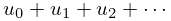
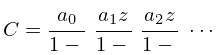
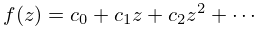
Every convergent, asymptotic, or formal series
| 3.10.3 | |||
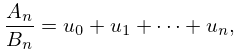
can be converted into a continued fraction of type (3.10.1), and with the property that the th convergent to is equal to the th partial sum of the series in (3.10.3), that is,
| 3.10.4 | |||
| . | |||
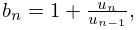
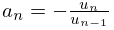
For instance, if none of the vanish, then we can define
| 3.10.5 | ||||
| , | ||||
| . | ||||
However, other continued fractions with the same limit may converge in a much larger domain of the complex plane than the fraction given by (3.10.4) and (3.10.5). For example, by converting the Maclaurin expansion of (4.24.3), we obtain a continued fraction with the same region of convergence (, ), whereas the continued fraction (4.25.4) converges for all except on the branch cuts from to and to .
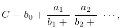
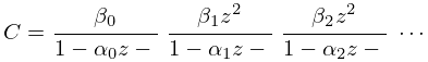
Stieltjes Fractions
A continued fraction of the form
| 3.10.6 | |||
is called a Stieltjes fraction (-fraction). We say that it corresponds to the formal power series
| 3.10.7 | |||
if the expansion of its th convergent in ascending powers of agrees with (3.10.7) up to and including the term in , .
Quotient-Difference Algorithm
For several special functions the -fractions are known explicitly, but in any case the coefficients can always be calculated from the power-series coefficients by means of the quotient-difference algorithm; see Table 3.10.1.
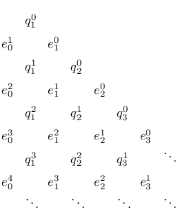 |
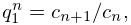
The first two columns in this table are defined by
| 3.10.8 | ||||
| , | ||||
| , | ||||
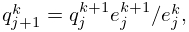
where the () appear in (3.10.7). We continue by means of the rhombus rule
| 3.10.9 | ||||
| , , | ||||
| , . | ||||
Then the coefficients of the -fraction (3.10.6) are given by
| 3.10.10 | ||||
The quotient-difference algorithm is frequently unstable and may require high-precision arithmetic or exact arithmetic. A more stable version of the algorithm is discussed in Stokes (1980). For applications to Bessel functions and Whittaker functions (Chapters 10 and 13), see Gargantini and Henrici (1967).
Jacobi Fractions
A continued fraction of the form
| 3.10.11 | |||
is called a Jacobi fraction (-fraction). We say that it is associated with the formal power series in (3.10.7) if the expansion of its th convergent in ascending powers of , agrees with (3.10.7) up to and including the term in , . For the same function , the convergent of the Jacobi fraction (3.10.11) equals the convergent of the Stieltjes fraction (3.10.6).
Examples of - and -Fractions
For special functions see §5.10 (gamma function), §7.9 (error function), §8.9 (incomplete gamma functions), §8.17(v) (incomplete beta function), §8.19(vii) (generalized exponential integral), §§10.10 and 10.33 (quotients of Bessel functions), §13.6 (quotients of confluent hypergeometric functions), §13.19 (quotients of Whittaker functions), and §15.7 (quotients of hypergeometric functions).
§3.10(iii) Numerical Evaluation of Continued Fractions
Forward Recurrence Algorithm
Backward Recurrence Algorithm
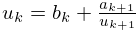
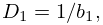
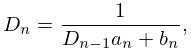
To compute the of (3.10.2) we perform the iterated divisions
| 3.10.12 | ||||
| , | ||||
| . | ||||
Then . To achieve a prescribed accuracy, either a priori knowledge is needed of the value of , or is determined by trial and error. In general this algorithm is more stable than the forward algorithm; see Jones and Thron (1974).
Forward Series Recurrence Algorithm
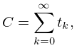
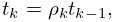
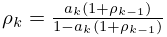
The continued fraction
| 3.10.13 | |||
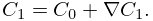
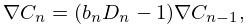
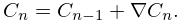
can be written in the form
| 3.10.14 | |||
where
| 3.10.15 | ||||
| , | ||||
| . | ||||
The th partial sum equals the th convergent of (3.10.13), . In contrast to the preceding algorithms in this subsection no scaling problems arise and no a priori information is needed.
Steed’s Algorithm
This forward algorithm achieves efficiency and stability in the computation of the convergents , and is related to the forward series recurrence algorithm. Again, no scaling problems arise and no a priori information is needed.
Let
| 3.10.16 | ||||
( is the backward difference operator.) Then for ,
| 3.10.17 | ||||
The recurrences are continued until is within a prescribed relative precision.
Alternatives to Steed’s algorithm are the Lentz algorithm Lentz (1976) and the modified Lentz algorithm Thompson and Barnett (1986).
For further information on the preceding algorithms, including convergence in the complex plane and methods for accelerating convergence, see Blanch (1964) and Lorentzen and Waadeland (1992, Chapter 3). For the evaluation of special functions by using continued fractions see Cuyt et al. (2008), Gautschi (1967, §1), Gil et al. (2007a, Chapter 6), and Wimp (1984, Chapter 4, §5). See also §§6.18(i), 7.22(i), 8.25(iv), 10.74(v), 14.32, 28.34(ii), 29.20(i), 30.16(i), 33.23(v).
