F. H. Jackson q-analog

SearchAdvancedHelp

(0.002 seconds)

11—20 of 353 matching pages

11: 16.11 Asymptotic Expansions

… ►For subsequent use we define two formal infinite series, $E_{p,q}(z)$ and $H_{p,q}(z)$, as follows: … ►It may be observed that $H_{p,q}(z)$ represents the sum of the residues of the poles of the integrand in (16.5.1) at $s=-a_j,-a_j-1,\mathrm{\dots }$, $j=1,\mathrm{\dots },p$, provided that these poles are all simple, that is, no two of the $a_j$ differ by an integer. (If this condition is violated, then the definition of $H_{p,q}(z)$ has to be modified so that the residues are those associated with the multiple poles. … ►The formal series (16.11.2) for $H_{q+1,q}(z)$ converges if $\left|z\right|>1$, and … ►Asymptotic expansions for the polynomials ${}_{p+2}{}^{}F_q^{}(-r,r+a_0,𝐚;𝐛;z)$ as $r\to \mathrm{\infty }$ through integer values are given in Fields and Luke (1963b, a) and Fields (1965).

12: 35.8 Generalized Hypergeometric Functions of Matrix Argument

… ►

§35.8(iii) ${}_3{}^{}F_2^{}$ Case

►

Kummer Transformation

… ►

Thomae Transformation

… ►Multidimensional Mellin–Barnes integrals are established in Ding et al. (1996) for the functions ${}_p{}^{}F_q^{}$ and ${}_{p+1}{}^{}F_p^{}$ of matrix argument. A similar result for the ${}_0{}^{}F_1^{}$ function of matrix argument is given in Faraut and Korányi (1994, p. 346). …

13: 16.4 Argument Unity

… ►The function ${}_{q+1}{}^{}F_q^{}(𝐚;𝐛;z)$ is well-poised if … ►The function ${}_{q+1}{}^{}F_q^{}$ with argument unity and general values of the parameters is discussed in Bühring (1992). … ►For generalizations involving ${}_{r+3}{}^{}F_{r+2}^{}$ functions see Kim et al. (2013). … ►There are two types of three-term identities for ${}_3{}^{}F_2^{}$’s. … ►Transformations for both balanced ${}_4{}^{}F_3^{}\left(1\right)$ and very well-poised ${}_7{}^{}F_6^{}\left(1\right)$ are included in Bailey (1964, pp. 56–63). …

14: 33.3 Graphics

… ►

§33.3(i) Line Graphs of the Coulomb Radial Functions $F_{\mathrm{\ell }}(\eta ,\rho )$ and $G_{\mathrm{\ell }}(\eta ,\rho )$

►

►►

Figure 33.3.1: $F_{\mathrm{\ell }}(\eta ,\rho )$, $G_{\mathrm{\ell }}(\eta ,\rho )$ with $\mathrm{\ell }=0$, $\eta =-2$. Magnify

►

►►

Figure 33.3.2: $F_{\mathrm{\ell }}(\eta ,\rho )$, $G_{\mathrm{\ell }}(\eta ,\rho )$ with $\mathrm{\ell }=0$, $\eta =0$. Magnify

… ►

33.3.1 $$M_{\mathrm{\ell }}(\eta ,\rho )={(F_{\mathrm{\ell }}^2(\eta ,\rho )+G_{\mathrm{\ell }}^2(\eta ,\rho ))}^{1/2}=\left|H_{\mathrm{\ell }}^{\pm }(\eta ,\rho )\right|.$$

ⓘ

Defines:

$M_{\mathrm{\ell }}(\eta ,\rho )$: envelope of Coulomb functions

Symbols:

$G_{\mathrm{\ell }}(\eta ,\rho )$: irregular Coulomb radial function, $H_{\mathrm{\ell }}^{\pm }(\eta ,\rho )$: irregular Coulomb radial functions, $F_{\mathrm{\ell }}(\eta ,\rho )$: regular Coulomb radial function, $\mathrm{\ell }$: nonnegative integer, $\rho$: nonnegative real variable and $\eta$: real parameter

Permalink:

http://dlmf.nist.gov/33.3.E1

Encodings:

pMML, png, TeX

See also:

Annotations for §33.3(i), §33.3 and Ch.33

… ►

§33.3(ii) Surfaces of the Coulomb Radial Functions $F_0(\eta ,\rho )$ and $G_0(\eta ,\rho )$

…

15: 33.23 Methods of Computation

… ►§33.8 supplies continued fractions for $F_{\mathrm{\ell }}^{\prime }/F_{\mathrm{\ell }}$ and $H_{\mathrm{\ell }}^{\pm }{}_{}{}^{\prime }/H_{\mathrm{\ell }}^{\pm }$. Combined with the Wronskians (33.2.12), the values of $F_{\mathrm{\ell }}$, $G_{\mathrm{\ell }}$, and their derivatives can be extracted. … ►Bardin et al. (1972) describes ten different methods for the calculation of $F_{\mathrm{\ell }}$ and $G_{\mathrm{\ell }}$, valid in different regions of the ($\eta ,\rho$)-plane. 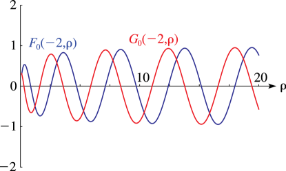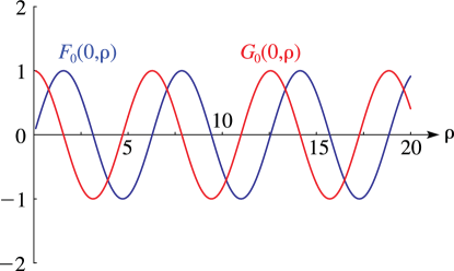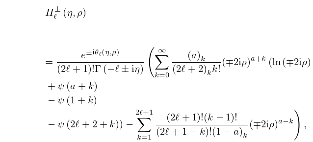… ►Hull and Breit (1959) and Barnett (1981b) give WKBJ approximations for $F_0$ and $G_0$ in the region inside the turning point: .

16: 33.6 Power-Series Expansions in $\rho$

… ►

33.6.1 $$F_{\mathrm{\ell }}(\eta ,\rho )=C_{\mathrm{\ell }}\left(\eta \right)\sum _{k=\mathrm{\ell }+1}^{\mathrm{\infty }}{A}_k^{\mathrm{\ell }}(\eta ){\rho }^k,$$

ⓘ

Symbols:

$C_{\mathrm{\ell }}\left(\eta \right)$: normalizing constant for Coulomb radial functions, $F_{\mathrm{\ell }}(\eta ,\rho )$: regular Coulomb radial function, $k$: nonnegative integer, $\mathrm{\ell }$: nonnegative integer, $\rho$: nonnegative real variable, $\eta$: real parameter and $A_{\mathrm{\ell }+1}^{\mathrm{\ell }}$: coefficient

A&S Ref:

14.1.4, 14.1.5

Referenced by:

§33.6

Permalink:

http://dlmf.nist.gov/33.6.E1

Encodings:

pMML, png, TeX

See also:

Annotations for §33.6 and Ch.33

►

33.6.2 $$F_{\mathrm{\ell }}^{\prime }(\eta ,\rho )=C_{\mathrm{\ell }}\left(\eta \right)\sum _{k=\mathrm{\ell }+1}^{\mathrm{\infty }}k{A}_k^{\mathrm{\ell }}(\eta ){\rho }^{k-1},$$

ⓘ

Symbols:

$C_{\mathrm{\ell }}\left(\eta \right)$: normalizing constant for Coulomb radial functions, $F_{\mathrm{\ell }}(\eta ,\rho )$: regular Coulomb radial function, $k$: nonnegative integer, $\mathrm{\ell }$: nonnegative integer, $\rho$: nonnegative real variable, $\eta$: real parameter and $A_{\mathrm{\ell }+1}^{\mathrm{\ell }}$: coefficient

A&S Ref:

14.1.4, 14.1.5

Referenced by:

§33.6

Permalink:

http://dlmf.nist.gov/33.6.E2

Encodings:

pMML, png, TeX

See also:

Annotations for §33.6 and Ch.33

… ►

33.6.4 $$A_k^{\mathrm{\ell }}(\eta )=\frac{{(-\mathrm{i})}^{k-\mathrm{\ell }-1}}{(k-\mathrm{\ell }-1)!}{}_2{}^{}F_1^{}(\mathrm{\ell }+1-k,\mathrm{\ell }+1-\mathrm{i}\eta ;2\mathrm{\ell }+2;2).$$

ⓘ

Symbols:

${}_2{}^{}F_1^{}(a,b;c;z)$: $=F(a,b;c;z)$ notation for Gauss’ hypergeometric function, $!$: factorial (as in $n!$), $\mathrm{i}$: imaginary unit, $k$: nonnegative integer, $\mathrm{\ell }$: nonnegative integer, $\eta$: real parameter and $A_{\mathrm{\ell }+1}^{\mathrm{\ell }}$: coefficient

Referenced by:

§33.6

Permalink:

http://dlmf.nist.gov/33.6.E4

Encodings:

pMML, png, TeX

See also:

Annotations for §33.6 and Ch.33

►

33.6.5 $$H_{\mathrm{\ell }}^{\pm }(\eta ,\rho )=\frac{{\mathrm{e}}^{\pm \mathrm{i}{\theta }_{\mathrm{\ell }}(\eta ,\rho )}}{(2\mathrm{\ell }+1)!\mathrm{\Gamma }\left(-\mathrm{\ell }\pm \mathrm{i}\eta \right)}\left(\sum _{k=0}^{\mathrm{\infty }}\frac{{\left(a\right)}_k}{{\left(2\mathrm{\ell }+2\right)}_{k}k!}{(\mp 2\mathrm{i}\rho )}^{a+k}\left(\ln \left(\mp 2\mathrm{i}\rho \right)+\psi \left(a+k\right)-\psi \left(1+k\right)-\psi \left(2\mathrm{\ell }+2+k\right)\right)-\sum _{k=1}^{2\mathrm{\ell }+1}\frac{(2\mathrm{\ell }+1)!(k-1)!}{(2\mathrm{\ell }+1-k)!{\left(1-a\right)}_k}{(\mp 2\mathrm{i}\rho )}^{a-k}\right),$$

ⓘ

Symbols:

${\theta }_{\mathrm{\ell }}(\eta ,\rho )$: phase of Coulomb functions, $\mathrm{\Gamma }\left(z\right)$: gamma function, ${\left(a\right)}_n$: Pochhammer’s symbol (or shifted factorial), $\psi \left(z\right)$: psi (or digamma) function, $\mathrm{e}$: base of natural logarithm, $!$: factorial (as in $n!$), $\mathrm{i}$: imaginary unit, $H_{\mathrm{\ell }}^{\pm }(\eta ,\rho )$: irregular Coulomb radial functions, $\ln z$: principal branch of logarithm function, $k$: nonnegative integer, $\mathrm{\ell }$: nonnegative integer, $\rho$: nonnegative real variable, $\eta$: real parameter and $a$: variable

A&S Ref:

14.1.14 (equivalent)

Referenced by:

§33.13, §33.6, §33.6, Erratum (V1.0.19) for Equation (33.6.5)

Permalink:

http://dlmf.nist.gov/33.6.E5

Encodings:

pMML, png, TeX

Errata (effective with 1.0.19):

On the right-hand side the factor in the denominator was incorrectly written as $\mathrm{\Gamma }\left(-\mathrm{\ell }+\mathrm{i}\eta \right)$. This has been corrected to $\mathrm{\Gamma }\left(-\mathrm{\ell }\pm \mathrm{i}\eta \right)$.

Reported 2018-05-15 by Ian Thompson

See also:

Annotations for §33.6 and Ch.33

… ►Corresponding expansions for $H_{\mathrm{\ell }}^{\pm }{}_{}{}^{\prime }(\eta ,\rho )$ can be obtained by combining (33.6.5) with (33.4.3) or (33.4.4).

17: 13.6 Relations to Other Functions

… ►

13.6.1 $$M(a,a,z)={\mathrm{e}}^z,$$

ⓘ

Symbols:

$M(a,b,z)$: $={}_1{}^{}F_1^{}(a;b;z)$ Kummer confluent hypergeometric function, $\mathrm{e}$: base of natural logarithm and $z$: complex variable

A&S Ref:

13.6.12

Referenced by:

§13.10(v)

Permalink:

http://dlmf.nist.gov/13.6.E1

Encodings:

pMML, png, TeX

See also:

Annotations for §13.6(i), §13.6 and Ch.13

… ►

13.6.16 $$M(-n,\frac{1}{2},z^2)={(-1)}^n\frac{n!}{(2n)!}{H}_{2n}\left(z\right),$$

ⓘ

Symbols:

$H_n\left(x\right)$: Hermite polynomial, $M(a,b,z)$: $={}_1{}^{}F_1^{}(a;b;z)$ Kummer confluent hypergeometric function, $!$: factorial (as in $n!$), $n$: nonnegative integer and $z$: complex variable

A&S Ref:

13.6.17

Referenced by:

§13.6(v)

Permalink:

http://dlmf.nist.gov/13.6.E16

Encodings:

pMML, png, TeX

See also:

Annotations for §13.6(v), §13.6(v), §13.6 and Ch.13

►

13.6.17 $$M(-n,\frac{3}{2},z^2)={(-1)}^n\frac{n!}{(2n+1)!2z}{H}_{2n+1}\left(z\right),$$

ⓘ

Symbols:

$H_n\left(x\right)$: Hermite polynomial, $M(a,b,z)$: $={}_1{}^{}F_1^{}(a;b;z)$ Kummer confluent hypergeometric function, $!$: factorial (as in $n!$), $n$: nonnegative integer and $z$: complex variable

A&S Ref:

13.6.18 (as corrected in later editions)

Permalink:

http://dlmf.nist.gov/13.6.E17

Encodings:

pMML, png, TeX

See also:

Annotations for §13.6(v), §13.6(v), §13.6 and Ch.13

… ►

13.6.21 $$U(a,b,z)=z^{-a}{}_2{}^{}F_0^{}(a,a-b+1;-;-z^{-1}).$$

ⓘ

Symbols:

${}_p{}^{}F_q^{}(a_1,\mathrm{\dots },a_p;b_1,\mathrm{\dots },b_q;z)$ or ${}_p{}^{}F_q^{}(\genfrac{}{}{0pt}{}{a_1,\mathrm{\dots },a_p}{b_1,\mathrm{\dots },b_q};z)$: alternatively ${}_p{}^{}F_q^{}(𝐚;𝐛;z)$ or ${}_p{}^{}F_q^{}(\genfrac{}{}{0pt}{}{𝐚}{𝐛};z)$
generalized hypergeometric function, $U(a,b,z)$: Kummer confluent hypergeometric function and $z$: complex variable

Referenced by:

§13.6(vi)

Permalink:

http://dlmf.nist.gov/13.6.E21

Encodings:

pMML, png, TeX

See also:

Annotations for §13.6(vi), §13.6 and Ch.13

►For the definition of ${}_2{}^{}F_0^{}(a,a-b+1;-;-z^{-1})$ when neither $a$ nor $a-b+1$ is a nonpositive integer see §16.5. …

18: 33.20 Expansions for Small $|ϵ|$

… ►

33.20.3 $$f(ϵ,\mathrm{\ell };r)=\sum _{k=0}^{\mathrm{\infty }}{ϵ}^k{𝖥}_k(\mathrm{\ell };r),$$

ⓘ

Symbols:

$f(ϵ,\mathrm{\ell };r)$: regular Coulomb function, $k$: nonnegative integer, $\mathrm{\ell }$: nonnegative integer, $r$: real variable, $ϵ$: real parameter and ${𝖥}_k(\mathrm{\ell };r)$: coefficient

Referenced by:

§33.20(ii)

Permalink:

http://dlmf.nist.gov/33.20.E3

Encodings:

pMML, png, TeX

See also:

Annotations for §33.20(ii), §33.20 and Ch.33

►where ►

33.20.4 $${𝖥}_k(\mathrm{\ell };r)=\sum _{p=2k}^{3k}{(2r)}^{(p+1)/2}{C}_{k,p}{J}_{2\mathrm{\ell }+1+p}\left(\sqrt{8r}\right),$$ $r>0$,

ⓘ

Symbols:

$J_{\nu }\left(z\right)$: Bessel function of the first kind, $k$: nonnegative integer, $\mathrm{\ell }$: nonnegative integer, $r$: real variable, ${𝖥}_k(\mathrm{\ell };r)$: coefficient and $C_{k,p}$: coefficients

Permalink:

http://dlmf.nist.gov/33.20.E4

Encodings:

pMML, png, TeX

See also:

Annotations for §33.20(ii), §33.20 and Ch.33

►

33.20.5 $${𝖥}_k(\mathrm{\ell };r)=\sum _{p=2k}^{3k}{(-1)}^{\mathrm{\ell }+1+p}{(2|r|)}^{(p+1)/2}{C}_{k,p}{I}_{2\mathrm{\ell }+1+p}\left(\sqrt{8|r|}\right),$$ .

ⓘ

Symbols:

$I_{\nu }\left(z\right)$: modified Bessel function of the first kind, $k$: nonnegative integer, $\mathrm{\ell }$: nonnegative integer, $r$: real variable, ${𝖥}_k(\mathrm{\ell };r)$: coefficient and $C_{k,p}$: coefficients

Permalink:

http://dlmf.nist.gov/33.20.E5

Encodings:

pMML, png, TeX

See also:

Annotations for §33.20(ii), §33.20 and Ch.33

… ►where $A(ϵ,\mathrm{\ell })$ is given by (33.14.11), (33.14.12), and …

19: 18.5 Explicit Representations

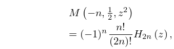
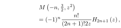
… ►In (18.5.4_5) see §26.11 for the Fibonacci numbers $F_n$. … ►In this equation $w(x)$ is as in Table 18.3.1, (reproduced in Table 18.5.1), and $F(x)$, ${\kappa }_n$ are as in Table 18.5.1. … ►For the definitions of ${}_2{}^{}F_1^{}$, ${}_1{}^{}F_1^{}$, and ${}_2{}^{}F_0^{}$ see §16.2. … ►

18.5.13 $$H_n\left(x\right)=n!\sum _{\mathrm{\ell }=0}^{\lfloor n/2\rfloor }\frac{{(-1)}^{\mathrm{\ell }}{(2x)}^{n-2\mathrm{\ell }}}{\mathrm{\ell }!(n-2\mathrm{\ell })!}={(2x)}^n{}_2{}^{}F_0^{}(\genfrac{}{}{0pt}{}{-\frac{1}{2}n,-\frac{1}{2}n+\frac{1}{2}}{-};-\frac{1}{x^2}).$$

ⓘ

Symbols:

${}_p{}^{}F_q^{}(a_1,\mathrm{\dots },a_p;b_1,\mathrm{\dots },b_q;z)$ or ${}_p{}^{}F_q^{}(\genfrac{}{}{0pt}{}{a_1,\mathrm{\dots },a_p}{b_1,\mathrm{\dots },b_q};z)$: alternatively ${}_p{}^{}F_q^{}(𝐚;𝐛;z)$ or ${}_p{}^{}F_q^{}(\genfrac{}{}{0pt}{}{𝐚}{𝐛};z)$
generalized hypergeometric function, $H_n\left(x\right)$: Hermite polynomial, $!$: factorial (as in $n!$), $\lfloor x\rfloor$: floor of $x$ , $\mathrm{\ell }$: nonnegative integer, $n$: nonnegative integer and $x$: real variable

A&S Ref:

22.3.10

Referenced by:

§18.17(v), §18.17(vii), §18.5(iii)

Permalink:

http://dlmf.nist.gov/18.5.E13

Encodings:

pMML, png, TeX

See also:

Annotations for §18.5(iii), §18.5(iii), §18.5 and Ch.18

… ►

$H_0\left(x\right)=1,$

…

20: 33.5 Limiting Forms for Small $\rho$, Small $|\eta |$, or Large $\mathrm{\ell }$

… ►

$F_{\mathrm{\ell }}(\eta ,\rho )\sim C_{\mathrm{\ell }}\left(\eta \right){\rho }^{\mathrm{\ell }+1},$

►

$F_{\mathrm{\ell }}^{\prime }(\eta ,\rho )\sim (\mathrm{\ell }+1)C_{\mathrm{\ell }}\left(\eta \right){\rho }^{\mathrm{\ell }}.$

… ►

$F_{\mathrm{\ell }}(0,\rho )=\rho {𝗃}_{\mathrm{\ell }}\left(\rho \right),$

… ►

$F_0(0,\rho )=\sin \rho ,$

… ►

$F_{\mathrm{\ell }}(\eta ,\rho )\sim C_{\mathrm{\ell }}\left(\eta \right){\rho }^{\mathrm{\ell }+1},$

…