33 Coulomb Functions Variables $r,\epsilon$ 33.13 Complex Variable and Parameters 33.15 Graphics

§33.14 Definitions and Basic Properties

Referenced by:: ¶ ‣ §33.22(ii)
Permalink:: http://dlmf.nist.gov/33.14

§33.14(i) Coulomb Wave Equation
§33.14(ii) Regular Solution $\mathop{f\/}\nolimits\!\left(\epsilon,\ell;r\right)$
§33.14(iii) Irregular Solution $\mathop{h\/}\nolimits\!\left(\epsilon,\ell;r\right)$
§33.14(iv) Solutions $\mathop{s\/}\nolimits\!\left(\epsilon,\ell;r\right)$ and $\mathop{c\/}\nolimits\!\left(\epsilon,\ell;r\right)$
§33.14(v) Wronskians

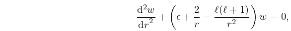
§33.14(i) Coulomb Wave Equation

Notes:: See Curtis (1964a, pp. ix–xxv), Seaton (1983), and Seaton (2002a, Eqs. 3, 4 and §2.3).
Keywords:: Coulomb functions: variables $r,\epsilon$ , Coulomb wave equation, singularities, turning points
Permalink:: http://dlmf.nist.gov/33.14.i

Another parametrization of (33.2.1) is given by

33.14.1 $\frac{{d}^{2}w}{{dr}^{2}}+\left(\epsilon+\frac{2}{r}-\frac{\ell(\ell+1)}{r^{2}% }\right)w=0,$

Symbols:: $\frac{df}{dx}$ : derivative of with respect to , $\ell$ : nonnegative integer, : real variable and $\epsilon$ : real parameter
Referenced by:: §33.23(iii)
Permalink:: http://dlmf.nist.gov/33.14.E1
Encodings:: TeX, pMML, png

where

33.14.2

$r=-\eta\rho,$

$\epsilon=1/\eta^{2}.$

Symbols:: : real variable, $\rho$ : nonnegative real variable, $\epsilon$ : real parameter and $\eta$ : real parameter
Permalink:: http://dlmf.nist.gov/33.14.E2
Encodings:: TeX, TeX, pMML, pMML, png, png

Again, there is a regular singularity at with indices $\ell+1$ and $-\ell$ , and an irregular singularity of rank 1 at $r=\infty$ . When $\epsilon>0$ the outer turning point is given by

33.14.3 $\mathop{r_{{\mathrm{tp}}}\/}\nolimits\!\left(\epsilon,\ell\right)=\left(\sqrt{% 1+\epsilon\ell(\ell+1)}-1\right)\Bigm/\epsilon;$

Defines:: $\mathop{r_{{\mathrm{tp}}}\/}\nolimits\!\left(\epsilon,\ell\right)$ : outer turning point for Coulomb functions
Symbols:: $\ell$ : nonnegative integer and $\epsilon$ : real parameter
Permalink:: http://dlmf.nist.gov/33.14.E3
Encodings:: TeX, pMML, png

compare (33.2.2).

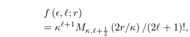
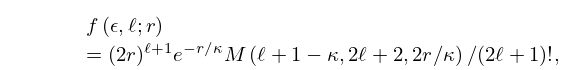
§33.14(ii) Regular Solution $\mathop{f\/}\nolimits\!\left(\epsilon,\ell;r\right)$

Notes:: See Seaton (2002a, Eqs. 7, 9, 14, 22).
Keywords:: Coulomb functions, Coulomb functions: variables $r,\epsilon$ , Whittaker functions, confluent hypergeometric functions
Referenced by:: §33.22(iii)
Permalink:: http://dlmf.nist.gov/33.14.ii

The function $\mathop{f\/}\nolimits\!\left(\epsilon,\ell;r\right)$ is recessive (§2.7(iii)) at , and is defined by

33.14.4 $\mathop{f\/}\nolimits\!\left(\epsilon,\ell;r\right)=\kappa^{{\ell+1}}\mathop{M% _{{\kappa,\ell+\frac{1}{2}}}\/}\nolimits\!\left(2r/\kappa\right)/(2\ell+1)!,$

Defines:: $\mathop{f\/}\nolimits\!\left(\epsilon,\ell;r\right)$ : regular Coulomb function
Symbols:: $\mathop{M_{{\kappa,\mu}}\/}\nolimits\!\left(z\right)$ : Whittaker confluent hypergeometric function, : : factorial, $\ell$ : nonnegative integer, : real variable, $\epsilon$ : real parameter and $\kappa$ : quantity
Permalink:: http://dlmf.nist.gov/33.14.E4
Encodings:: TeX, pMML, png

or equivalently

33.14.5 $\mathop{f\/}\nolimits\!\left(\epsilon,\ell;r\right)=(2r)^{{\ell+1}}e^{{-r/% \kappa}}\mathop{M\/}\nolimits\!\left(\ell+1-\kappa,2\ell+2,2r/\kappa\right)/{(% 2\ell+1)!},$

Symbols:: $\mathop{f\/}\nolimits\!\left(\epsilon,\ell;r\right)$ : regular Coulomb function, $\mathop{M\/}\nolimits\!\left(a,b,z\right)$ : Kummer confluent hypergeometric function, : base of exponential function, : : factorial, $\ell$ : nonnegative integer, : real variable, $\epsilon$ : real parameter and $\kappa$ : quantity
Permalink:: http://dlmf.nist.gov/33.14.E5
Encodings:: TeX, pMML, png

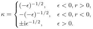
where $\mathop{M_{{\kappa,\mu}}\/}\nolimits\!\left(z\right)$ and $\mathop{M\/}\nolimits\!\left(a,b,z\right)$ are defined in §§13.14(i) and 13.2(i), and

33.14.6 $\kappa=\begin{cases}(-\epsilon)^{{-1/2}},&\epsilon<0,r>0,\\ -(-\epsilon)^{{-1/2}},&\epsilon<0,r<0,\\ \pm i\epsilon^{{-1/2}},&\epsilon>0.\end{cases}$

Symbols:: : real variable, $\epsilon$ : real parameter and $\kappa$ : quantity
Referenced by:: §33.14(ii), §33.14(iii), §33.14(iv), §33.16(v), §33.19
Permalink:: http://dlmf.nist.gov/33.14.E6
Encodings:: TeX, pMML, png

The choice of sign in the last line of (33.14.6) is immaterial: the same function $\mathop{f\/}\nolimits\!\left(\epsilon,\ell;r\right)$ is obtained. This is a consequence of Kummer’s transformation (§13.2(vii)).

$\mathop{f\/}\nolimits\!\left(\epsilon,\ell;r\right)$ is real and an analytic function of in the interval $-\infty<r<\infty$ , and it is also an analytic function of $\epsilon$ when $-\infty<\epsilon<\infty$ . This includes $\epsilon=0$ , hence $\mathop{f\/}\nolimits\!\left(\epsilon,\ell;r\right)$ can be expanded in a convergent power series in $\epsilon$ in a neighborhood of $\epsilon=0$ (§33.20(ii)).

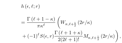
§33.14(iii) Irregular Solution $\mathop{h\/}\nolimits\!\left(\epsilon,\ell;r\right)$

Notes:: See Seaton (2002a, Eqs. 47, 49, 109, 131).
Keywords:: Coulomb functions, Coulomb functions: variables $r,\epsilon$ , Whittaker functions, confluent hypergeometric functions
Referenced by:: §33.22(iii), §33.23(iii), §33.23(iv)
Permalink:: http://dlmf.nist.gov/33.14.iii

For nonzero values of $\epsilon$ and the function $\mathop{h\/}\nolimits\!\left(\epsilon,\ell;r\right)$ is defined by

33.14.7 $\mathop{h\/}\nolimits\!\left(\epsilon,\ell;r\right)=\frac{\mathop{\Gamma\/}% \nolimits\!\left(\ell+1-\kappa\right)}{\pi\kappa^{\ell}}\left(\mathop{W_{{% \kappa,\ell+\frac{1}{2}}}\/}\nolimits\!\left(2r/\kappa\right)+(-1)^{\ell}S(% \epsilon,r)\frac{\mathop{\Gamma\/}\nolimits\!\left(\ell+1+\kappa\right)}{2(2% \ell+1)!}\mathop{M_{{\kappa,\ell+\frac{1}{2}}}\/}\nolimits\!\left(2r/\kappa% \right)\right),$

Defines:: $\mathop{h\/}\nolimits\!\left(\epsilon,\ell;r\right)$ : irregular Coulomb function
Symbols:: $\mathop{\Gamma\/}\nolimits\!\left(z\right)$ : gamma function, $\mathop{M_{{\kappa,\mu}}\/}\nolimits\!\left(z\right)$ : Whittaker confluent hypergeometric function, $\mathop{W_{{\kappa,\mu}}\/}\nolimits\!\left(z\right)$ : Whittaker confluent hypergeometric function, : : factorial, $\ell$ : nonnegative integer, : real variable, $\epsilon$ : real parameter, $\kappa$ : quantity and $S(\epsilon,r)$ : function
Permalink:: http://dlmf.nist.gov/33.14.E7
Encodings:: TeX, pMML, png

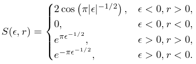
where $\kappa$ is given by (33.14.6) and

33.14.8 $S(\epsilon,r)=\begin{cases}2\mathop{\cos\/}\nolimits\!\left(\pi|\epsilon|^{{-1% /2}}\right),&\epsilon<0,r>0,\\ 0,&\epsilon<0,r<0,\\ e^{{\pi\epsilon^{{-1/2}}}},&\epsilon>0,r>0,\\ e^{{-\pi\epsilon^{{-1/2}}}},&\epsilon>0,r<0.\end{cases}$

Symbols:: $\mathop{\cos\/}\nolimits z$ : cosine function, : base of exponential function, : real variable, $\epsilon$ : real parameter and $S(\epsilon,r)$ : function
Permalink:: http://dlmf.nist.gov/33.14.E8
Encodings:: TeX, pMML, png

(Again, the choice of the ambiguous sign in the last line of (33.14.6) is immaterial.)

$\mathop{h\/}\nolimits\!\left(\epsilon,\ell;r\right)$ is real and an analytic function of each of and $\epsilon$ in the intervals $-\infty<r<\infty$ and $-\infty<\epsilon<\infty$ , except when or $\epsilon=0$ .

§33.14(iv) Solutions $\mathop{s\/}\nolimits\!\left(\epsilon,\ell;r\right)$ and $\mathop{c\/}\nolimits\!\left(\epsilon,\ell;r\right)$

Notes:: See Seaton (2002a, Eqs. 113–115, 122–125). For (33.14.11) and (33.14.12) see Humblet (1985, Eqs. 1.4a,b), Seaton (1982, Eq. 2.4.4).
Keywords:: Coulomb functions: variables $r,\epsilon$
Referenced by:: ¶ ‣ §1.17(ii)
Permalink:: http://dlmf.nist.gov/33.14.iv

The functions $\mathop{s\/}\nolimits\!\left(\epsilon,\ell;r\right)$ and $\mathop{c\/}\nolimits\!\left(\epsilon,\ell;r\right)$ are defined by

33.14.9

$\mathop{s\/}\nolimits\!\left(\epsilon,\ell;r\right)=(B(\epsilon,\ell)/2)^{{1/2% }}\mathop{f\/}\nolimits\!\left(\epsilon,\ell;r\right),$

$\mathop{c\/}\nolimits\!\left(\epsilon,\ell;r\right)=(2B(\epsilon,\ell))^{{-1/2% }}\mathop{h\/}\nolimits\!\left(\epsilon,\ell;r\right),$

Defines:: $\mathop{c\/}\nolimits\!\left(\epsilon,\ell;r\right)$ : irregular Coulomb function and $\mathop{s\/}\nolimits\!\left(\epsilon,\ell;r\right)$ : regular Coulomb function
Symbols:: $\mathop{f\/}\nolimits\!\left(\epsilon,\ell;r\right)$ : regular Coulomb function, $\mathop{h\/}\nolimits\!\left(\epsilon,\ell;r\right)$ : irregular Coulomb function, $\ell$ : nonnegative integer, : real variable, $\epsilon$ : real parameter and $B(\epsilon,\ell)$ : function
Referenced by:: §33.16(iv), §33.16(v)
Permalink:: http://dlmf.nist.gov/33.14.E9
Encodings:: TeX, TeX, pMML, pMML, png, png

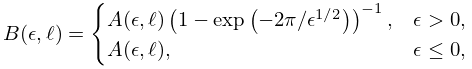
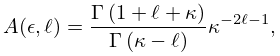
provided that $\ell<(-\epsilon)^{{-1/2}}$ when $\epsilon<0$ , where

33.14.10 $B(\epsilon,\ell)=\begin{cases}A(\epsilon,\ell)\left(1-\mathop{\exp\/}\nolimits% \!\left(-2\pi/\epsilon^{{1/2}}\right)\right)^{{-1}},&\epsilon>0,\\ A(\epsilon,\ell),&\epsilon\leq 0,\end{cases}$

Symbols:: $\mathop{\exp\/}\nolimits z$ : exponential function, $\ell$ : nonnegative integer, $\epsilon$ : real parameter, $B(\epsilon,\ell)$ : function and $A(\epsilon,\ell)$ : function
Permalink:: http://dlmf.nist.gov/33.14.E10
Encodings:: TeX, pMML, png

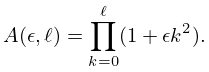
and

33.14.11 $A(\epsilon,\ell)=\prod_{{k=0}}^{\ell}(1+\epsilon k^{2}).$

Symbols:: : nonnegative integer, $\ell$ : nonnegative integer, $\epsilon$ : real parameter and $A(\epsilon,\ell)$ : function
Referenced by:: §33.14(iv), §33.16(ii), §33.16(iii), §33.19, §33.20(iii)
Permalink:: http://dlmf.nist.gov/33.14.E11
Encodings:: TeX, pMML, png

An alternative formula for $A(\epsilon,\ell)$ is

33.14.12 $A(\epsilon,\ell)=\frac{\mathop{\Gamma\/}\nolimits\!\left(1+\ell+\kappa\right)}% {\mathop{\Gamma\/}\nolimits\!\left(\kappa-\ell\right)}\kappa^{{-2\ell-1}},$

Symbols:: $\mathop{\Gamma\/}\nolimits\!\left(z\right)$ : gamma function, $\ell$ : nonnegative integer, $\epsilon$ : real parameter, $\kappa$ : quantity and $A(\epsilon,\ell)$ : function
Referenced by:: §33.14(iv), §33.16(ii), §33.16(iii), §33.16(v), §33.19, §33.20(iii)
Permalink:: http://dlmf.nist.gov/33.14.E12
Encodings:: TeX, pMML, png

the choice of sign in the last line of (33.14.6) again being immaterial.

When $\epsilon<0$ and $\ell>(-\epsilon)^{{-1/2}}$ the quantity $A(\epsilon,\ell)$ may be negative, causing $\mathop{s\/}\nolimits\!\left(\epsilon,\ell;r\right)$ and $\mathop{c\/}\nolimits\!\left(\epsilon,\ell;r\right)$ to become imaginary.

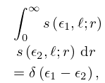
The function $\mathop{s\/}\nolimits\!\left(\epsilon,\ell;r\right)$ has the following properties:

33.14.13 $\int_{0}^{\infty}\mathop{s\/}\nolimits\!\left(\epsilon_{1},\ell;r\right)% \mathop{s\/}\nolimits\!\left(\epsilon_{2},\ell;r\right)dr=\mathop{\delta\/}% \nolimits\!\left(\epsilon_{1}-\epsilon_{2}\right),$

Symbols:: $\mathop{s\/}\nolimits\!\left(\epsilon,\ell;r\right)$ : regular Coulomb function, $\mathop{\delta\/}\nolimits\!\left(x-a\right)$ : Dirac delta (or Dirac delta function), : differential of , $\int$ : integral, $\ell$ : nonnegative integer, : real variable and $\epsilon$ : real parameter
Permalink:: http://dlmf.nist.gov/33.14.E13
Encodings:: TeX, pMML, png

where the right-hand side is the Dirac delta (§1.17). When $\epsilon=-1/n^{2}$ , $n=\ell+1,\ell+2,\dots$ , $\mathop{s\/}\nolimits\!\left(\epsilon,\ell;r\right)$ is $\mathop{\exp\/}\nolimits\!\left(-r/n\right)$ times a polynomial in , and

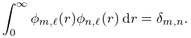
33.14.14 $\phi_{{n,\ell}}(r)=(-1)^{{\ell+1+n}}(2/n^{3})^{{1/2}}\mathop{s\/}\nolimits\!% \left(-1/n^{2},\ell;r\right)$

Symbols:: $\mathop{s\/}\nolimits\!\left(\epsilon,\ell;r\right)$ : regular Coulomb function, $\ell$ : nonnegative integer, : real variable and $\phi_{{n,\ell}}(r)$ : function
Referenced by:: §33.22(v)
Permalink:: http://dlmf.nist.gov/33.14.E14
Encodings:: TeX, pMML, png

satisfies

33.14.15 $\int_{0}^{\infty}\phi_{{n,\ell}}^{2}(r)dr=1.$

Symbols:: : differential of , $\int$ : integral, $\ell$ : nonnegative integer, : real variable and $\phi_{{n,\ell}}(r)$ : function
Permalink:: http://dlmf.nist.gov/33.14.E15
Encodings:: TeX, pMML, png

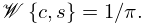
§33.14(v) Wronskians

Notes:: See Seaton (2002a, Eqs. 51, 116).
Keywords:: Coulomb functions: variables $r,\epsilon$
Permalink:: http://dlmf.nist.gov/33.14.v

With arguments $\epsilon,\ell,r$ suppressed,

33.14.16

$\mathop{\mathscr{W}\/}\nolimits\left\{\mathop{h\/}\nolimits,\mathop{f\/}% \nolimits\right\}=2/\pi,$

$\mathop{\mathscr{W}\/}\nolimits\left\{\mathop{c\/}\nolimits,\mathop{s\/}% \nolimits\right\}=1/\pi.$

Symbols:: $\mathop{c\/}\nolimits\!\left(\epsilon,\ell;r\right)$ : irregular Coulomb function, $\mathop{f\/}\nolimits\!\left(\epsilon,\ell;r\right)$ : regular Coulomb function, $\mathop{h\/}\nolimits\!\left(\epsilon,\ell;r\right)$ : irregular Coulomb function, $\mathop{s\/}\nolimits\!\left(\epsilon,\ell;r\right)$ : regular Coulomb function and $\mathop{\mathscr{W}\/}\nolimits$ : Wronskian
Permalink:: http://dlmf.nist.gov/33.14.E16
Encodings:: TeX, TeX, pMML, pMML, png, png

© 2010–2013 NIST / Privacy Policy / Disclaimer / Feedback; Version 1.0.6; Release date 2013-05-06 Math-Image version (See MathML) . A Printed Companionis available. 33.13 Complex Variable and Parameters 33.15 Graphics

§33.14 Definitions and Basic Properties

Contents

§33.14(i) Coulomb Wave Equation

§33.14(ii) Regular Solution

§33.14(iii) Irregular Solution

§33.14(iv) Solutions and

§33.14(v) Wronskians

§33.14(ii) Regular Solution $\mathop{f\/}\nolimits\!\left(\epsilon,\ell;r\right)$

§33.14(iii) Irregular Solution $\mathop{h\/}\nolimits\!\left(\epsilon,\ell;r\right)$

§33.14(iv) Solutions $\mathop{s\/}\nolimits\!\left(\epsilon,\ell;r\right)$ and $\mathop{c\/}\nolimits\!\left(\epsilon,\ell;r\right)$