.足球世界杯开球_『wn4.com_』世界杯输了要赔钱吗_w6n2c9o_2022年11月29日2时54分22秒_ic6k0s0ic
(0.003 seconds)
21—30 of 789 matching pages
21: Bibliography
…
►
On the zeros of confluent hypergeometric functions. III. Characterization by means of nonlinear equations.
Lett. Nuovo Cimento (2) 29 (11), pp. 353–358.
…
►
Uniform asymptotic expansions for exponential integrals and Bickley functions
.
ACM Trans. Math. Software 9 (4), pp. 467–479.
…
►
Special value of the hypergeometric function and connection formulae among asymptotic expansions.
J. Indian Math. Soc. (N.S.) 51, pp. 161–221.
…
►
Normal forms of functions near degenerate critical points, the Weyl groups and Lagrangian singularities.
Funkcional. Anal. i Priložen. 6 (4), pp. 3–25 (Russian).
►
Normal forms of functions in the neighborhood of degenerate critical points.
Uspehi Mat. Nauk 29 (2(176)), pp. 11–49 (Russian).
…
22: 24.20 Tables
…
►Abramowitz and Stegun (1964, Chapter 23) includes exact values of , , ; , , , , 20D; , , 18D.
►Wagstaff (1978) gives complete prime factorizations of and for and , respectively.
…
►For information on tables published before 1961 see Fletcher et al. (1962, v. 1, §4) and Lebedev and Fedorova (1960, Chapters 11 and 14).
23: 3.11 Approximation Techniques
…
►Beginning with , , we apply
…
►With , the last equations give as the solution of a system of linear equations.
…
►(3.11.29) is a system of linear equations for the coefficients .
…
►With this choice of and , the corresponding sum (3.11.32) vanishes.
…
►Two are endpoints: and ; the other points and are control points.
…
24: Bibliography K
…
►
The asymptotic expansion of a hypergeometric function
.
Math. Comp. 26 (120), pp. 963.
…
►
An extension of Saalschütz’s summation theorem for the series
.
Integral Transforms Spec. Funct. 24 (11), pp. 916–921.
…
►
On the complex zeros of for real or complex order.
J. Comput. Appl. Math. 40 (3), pp. 337–344.
…
►
Fractional integral and generalized Stieltjes transforms for hypergeometric functions as transmutation operators.
SIGMA Symmetry Integrability Geom. Methods Appl. 11, pp. Paper 074, 22.
…
►
Some special cases of the generalized hypergeometric function
.
J. Comput. Appl. Math. 78 (1), pp. 79–95.
…
25: Bibliography O
…
►
Studies on the Painlevé equations. III. Second and fourth Painlevé equations, and
.
Math. Ann. 275 (2), pp. 221–255.
►
Studies on the Painlevé equations. I. Sixth Painlevé equation
.
Ann. Mat. Pura Appl. (4) 146, pp. 337–381.
►
Studies on the Painlevé equations. II. Fifth Painlevé equation
.
Japan. J. Math. (N.S.) 13 (1), pp. 47–76.
►
Studies on the Painlevé equations. IV. Third Painlevé equation
.
Funkcial. Ekvac. 30 (2-3), pp. 305–332.
…
►
Algorithm 22: Riccati-Bessel functions of first and second kind.
Comm. ACM 3 (11), pp. 600–601.
…
26: 4.17 Special Values and Limits
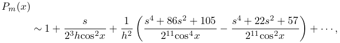
27: 28.8 Asymptotic Expansions for Large
…
►Also let and (§18.3).
…
►
…
►
28.8.11
…
►The approximations are expressed in terms of Whittaker functions and with ; compare §2.8(vi).
…
►Subsequently the asymptotic solutions involving either elementary or Whittaker functions are identified in terms of the Floquet solutions (§28.12(ii)) and modified Mathieu functions (§28.20(iii)).
…
28: Bibliography H
…
►
La -conjecture de Macdonald-Morris pour
.
C. R. Acad. Sci. Paris Sér. I Math. 303 (6), pp. 211–213 (French).
…
►
25D Table of the First One Hundred Values of ,, ,,,
.
Technical report
Department of Physics, Worcester Polytechnic Institute, Worcester, MA.
…
►
Inverse virial symmetry of diatomic potential curves.
J. Chem. Phys. 109 (1), pp. 11–19.
…
►
Error bounds for asymptotic approximations of zeros of Hankel functions occurring in diffraction problems.
J. Mathematical Phys. 11 (8), pp. 2501–2504.
…
►
Algorithm 571: Statistics for von Mises’ and Fisher’s distributions of directions: , and their inverses [S14].
ACM Trans. Math. Software 7 (2), pp. 233–238.
…
29: 18.38 Mathematical Applications
…
►For the generalized hypergeometric function see (16.2.1).
…
►Define operators and acting on symmetric Laurent polynomials by ( given by (18.28.6_2)) and .
…commutes with , that is , and satisfies
…where is a constant with explicit expression in terms of and given in Koornwinder (2007a, (2.8)).
►The abstract associative algebra with generators and relations (18.38.4), (18.38.6) and with the constants in (18.38.6) not yet specified, is called the Zhedanov algebra or Askey–Wilson algebra AW(3).
…
