.樊振东世界杯冠军_『wn4.com_』cntv能否看世界杯_w6n2c9o_2022年11月29日22时14分2秒_2kukma4ks_gov_hk
(0.007 seconds)
11—20 of 848 matching pages
11: 26.16 Multiset Permutations
…
►Let be the multiset that has copies of , .
denotes the set of permutations of for all distinct orderings of the integers.
The number of elements in is the multinomial coefficient (§26.4) .
…
►The
-multinomial coefficient is defined in terms of Gaussian polynomials (§26.9(ii)) by
…and again with we have
…
12: 26.4 Lattice Paths: Multinomial Coefficients and Set Partitions
…
►
is the number of ways of placing distinct objects into labeled boxes so that there are objects in the th box.
…
►These are given by the following equations in which are nonnegative integers such that
… is the number of permutations of with cycles of length 1, cycles of length 2, , and cycles of length :
…For each all possible values of are covered.
…
►where the summation is over all nonnegative integers such that .
…
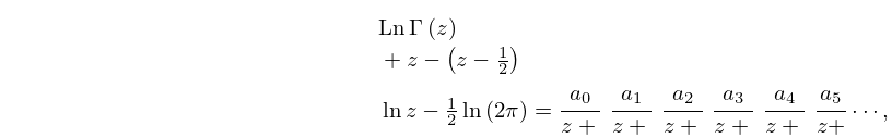
13: 5.10 Continued Fractions
14: 18.8 Differential Equations
15: 25.20 Approximations
…
►
•
►
•
►
•
►
•
►
•
Cody et al. (1971) gives rational approximations for in the form of quotients of polynomials or quotients of Chebyshev series. The ranges covered are , , , . Precision is varied, with a maximum of 20S.
Piessens and Branders (1972) gives the coefficients of the Chebyshev-series expansions of and , , for (23D).
16: 21.1 Special Notation
…
►
►
…
►The function is also commonly used; see, for example, Belokolos et al. (1994, §2.5), Dubrovin (1981), and Fay (1973, Chapter 1).
| positive integers. | |
| … | |
| Transpose of . | |
| … | |
| . | |
| … | |
| set of all elements of the form “”. | |
| set of all elements of , modulo elements of . Thus two elements of are equivalent if they are both in and their difference is in . (For an example see §20.12(ii).) | |
| … | |
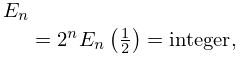
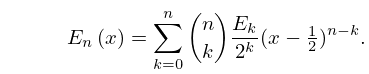
17: 24.2 Definitions and Generating Functions
18: 10.75 Tables
…
►
•
…
►
•
…
►
•
…
►
•
…
►
•
…
Makinouchi (1966) tabulates all values of and in the interval , with at least 29S. These are for , 10, 20; , ; with and , except for .
Abramowitz and Stegun (1964, Chapter 11) tabulates , , , 10D; , , , 8D.
Leung and Ghaderpanah (1979), tabulates all zeros of the principal value of , for , 29S.
Abramowitz and Stegun (1964, Chapter 11) tabulates , , , 7D; , , , 6D.
19: 26.12 Plane Partitions
…
►The number of self-complementary plane partitions in is
…in it is
…in it is
…
►The notation denotes the sum over all plane partitions contained in , and denotes the number of elements in .
…
►where is the sum of the squares of the divisors of .
…
20: Bibliography
…
►
Asymptotic expansions of spheroidal wave functions.
J. Math. Phys. Mass. Inst. Tech. 28, pp. 195–199.
…
►
On the zeros of confluent hypergeometric functions. III. Characterization by means of nonlinear equations.
Lett. Nuovo Cimento (2) 29 (11), pp. 353–358.
…
►
Transformations of the ranks and algebraic solutions of the sixth Painlevé equation.
Comm. Math. Phys. 228 (1), pp. 151–176.
…
►
Special value of the hypergeometric function and connection formulae among asymptotic expansions.
J. Indian Math. Soc. (N.S.) 51, pp. 161–221.
…
►
Normal forms of functions in the neighborhood of degenerate critical points.
Uspehi Mat. Nauk 29 (2(176)), pp. 11–49 (Russian).
…
