§1.10 Functions of a Complex Variable
Contents
- §1.10(i) Taylor’s Theorem for Complex Variables
- §1.10(ii) Analytic Continuation
- §1.10(iii) Laurent Series
- §1.10(iv) Residue Theorem
- §1.10(v) Maximum-Modulus Principle
- §1.10(vi) Multivalued Functions
- §1.10(vii) Inverse Functions
- §1.10(viii) Functions Defined by Contour Integrals
- §1.10(ix) Infinite Products
- §1.10(x) Infinite Partial Fractions
- §1.10(xi) Generating Functions
§1.10(i) Taylor’s Theorem for Complex Variables
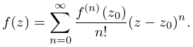
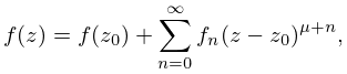
Let be analytic on the disk . Then
| 1.10.1 | |||
The right-hand side is the Taylor series for at , and its radius of convergence is at least .
Examples
Zeros
An analytic function has a zero of order (or multiplicity) () at if the first nonzero coefficient in its Taylor series at is that of . When the zero is simple.
§1.10(ii) Analytic Continuation
Let be analytic in a domain . If , analytic in , equals on an arc in , or on just an infinite number of points with a limit point in , then they are equal throughout and is called an analytic continuation of . We write , to signify this continuation.
Suppose , , is an arc and . Suppose the subarc , is contained in a domain , . The function on is said to be analytically continued along the path , , if there is a chain , .
Analytic continuation is a powerful aid in establishing transformations or functional equations for complex variables, because it enables the problem to be reduced to: (a) deriving the transformation (or functional equation) with real variables; followed by (b) finding the domain on which the transformed function is analytic.
Schwarz Reflection Principle
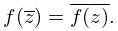
Let be a simple closed contour consisting of a segment of the real axis and a contour in the upper half-plane joining the ends of . Also, let be analytic within , continuous within and on , and real on . Then can be continued analytically across by reflection, that is,
| 1.10.5 | |||
§1.10(iii) Laurent Series
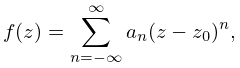
Suppose is analytic in the annulus , , and . Then
| 1.10.6 | |||
where
| 1.10.7 | |||
and the integration contour is described once in the positive sense. The series (1.10.6) converges uniformly and absolutely on compact sets in the annulus.
Let , so that the annulus becomes the punctured neighborhood : , and assume that is analytic in , but not at . Then is an isolated singularity of . This singularity is removable if for all , and in this case the Laurent series becomes the Taylor series. Next, is a pole if for at least one, but only finitely many, negative . If is the first negative integer (counting from ) with , then is a pole of order (or multiplicity) . Lastly, if for infinitely many negative , then is an isolated essential singularity.
The singularities of at infinity are classified in the same way as the singularities of at .
An isolated singularity is always removable when exists, for example at .
The coefficient of in the Laurent series for is called the residue of at , and denoted by , , or (when there is no ambiguity) .
A function whose only singularities, other than the point at infinity, are poles is called a meromorphic function. If the poles are infinite in number, then the point at infinity is called an essential singularity: it is the limit point of the poles.
Picard’s Theorem
In any neighborhood of an isolated essential singularity, however small, an analytic function assumes every value in with at most one exception.
§1.10(iv) Residue Theorem
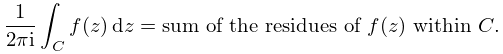
If is analytic within a simple closed contour , and continuous within and on —except in both instances for a finite number of singularities within —then
| 1.10.8 | |||
Here and elsewhere in this subsection the path is described in the positive sense.
Phase (or Argument) Principle
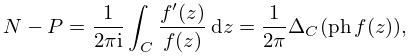
If the singularities within are poles and is analytic and nonvanishing on , then
| 1.10.9 | |||
where and are respectively the numbers of zeros and poles, counting multiplicity, of within , and is the change in any continuous branch of as passes once around in the positive sense. For examples of applications see Olver (1997b, pp. 252–254).
In addition,
| 1.10.10 | |||
each location again being counted with multiplicity equal to that of the corresponding zero or pole.
Rouché’s Theorem
If and are analytic on and inside a simple closed contour , and on , then and have the same number of zeros inside .
§1.10(v) Maximum-Modulus Principle
Analytic Functions
If is analytic in a domain , and for all , then is a constant in .
Let be a bounded domain with boundary and let . If is continuous on and analytic in , then attains its maximum on .
Harmonic Functions
If is harmonic in , , and for all , then is constant in . Moreover, if is bounded and is continuous on and harmonic in , then is maximum at some point on .
Schwarz’s Lemma
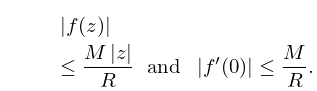
In , if is analytic, , and , then
| 1.10.11 | |||
Equalities hold iff , where is a constant such that .
§1.10(vi) Multivalued Functions
Functions which have more than one value at a given point are called multivalued (or many-valued) functions. Let be a multivalued function and be a domain. If we can assign a unique value to at each point of , and is analytic on , then is a branch of .
Example
is two-valued for . If and , then one branch is , the other branch is , with in both cases. Similarly if , then one branch is , the other branch is , with in both cases.
A cut domain is one from which the points on finitely many nonintersecting simple contours (§1.9(iii)) have been removed. Each contour is called a cut. A cut neighborhood is formed by deleting a ray emanating from the center. (Or more generally, a simple contour that starts at the center and terminates on the boundary.)
Suppose is multivalued and is a point such that there exists a branch of in a cut neighborhood of , but there does not exist a branch of in any punctured neighborhood of . Then is a branch point of . For example, is a branch point of .
Branches can be constructed in two ways:
(a) By introducing appropriate cuts from the branch points and restricting to be single-valued in the cut plane (or domain).
(b) By specifying the value of at a point (not a branch point), and requiring to be continuous on any path that begins at and does not pass through any branch points or other singularities of .
If the path circles a branch point at , times in the positive sense, and returns to without encircling any other branch point, then its value is denoted conventionally as .
Example
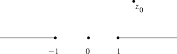
Let and be real or complex numbers that are not integers. The function is many-valued with branch points at . Branches of can be defined, for example, in the cut plane obtained from by removing the real axis from to and from to ; see Figure 1.10.1. One such branch is obtained by assigning and their principal values (§4.2(iv)).

Alternatively, take to be any point in and set where the logarithms assume their principal values. (Thus if is in the interval , then the logarithms are real.) Then the value of at any other point is obtained by analytic continuation.
Thus if is continued along a path that circles times in the positive sense and returns to without circling , then . If the path also circles times in the clockwise or negative sense before returning to , then the value of becomes .
§1.10(vii) Inverse Functions
Lagrange Inversion Theorem
Suppose is analytic at , , and . Then the equation
| 1.10.12 | |||
has a unique solution analytic at , and
| 1.10.13 | |||
in a neighborhood of , where is the residue of at . (In other words is the coefficient of in the Laurent expansion of in powers of ; compare §1.10(iii).)
Furthermore, if is analytic at , then
| 1.10.14 | |||
where is the residue of at .
Extended Inversion Theorem
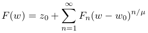
Suppose that
| 1.10.15 | |||
where , , and the series converges in a neighborhood of . (For example, when is an integer has a zero of order at .) Let . Then (1.10.12) has a solution , where
| 1.10.16 | |||
in a neighborhood of , being the residue of at .
§1.10(viii) Functions Defined by Contour Integrals
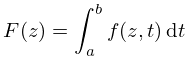
Let be a domain and be a closed finite segment of the real axis. Assume that for each , is an analytic function of in , and also that is a continuous function of both variables. Then
| 1.10.18 | |||
is analytic in and its derivatives of all orders can be found by differentiating under the sign of integration.
This result is also true when , or when has a singularity at , with the following conditions. For each , is analytic in ; is a continuous function of both variables when and ; the integral (1.10.18) converges at , and this convergence is uniform with respect to in every compact subset of .
The last condition means that given () there exists a number that is independent of and is such that
| 1.10.19 | |||
for all and all ; compare §1.5(iv).
-test
If for and converges, then the integral (1.10.18) converges uniformly and absolutely in .
§1.10(ix) Infinite Products
Let . If for some , as , then we say that the infinite product converges. (The integer may be greater than one to allow for a finite number of zero factors.) The convergence of the product is absolute if converges. The product , with for all , converges iff converges; and it converges absolutely iff converges.
Suppose , , a domain. The convergence of the infinite product is uniform if the sequence of partial products converges uniformly.
-test
Suppose that are analytic functions in . If there is an , independent of , such that
| 1.10.20 | |||
| , | |||
and
| 1.10.21 | |||
then the product converges uniformly to an analytic function in , and only when at least one of the factors is zero in . This conclusion remains true if, in place of (1.10.20), for all , and again .
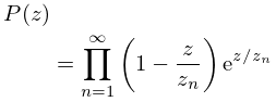
Weierstrass Product
If is a sequence such that is convergent, then
| 1.10.22 | |||
is an entire function with zeros at .
§1.10(x) Infinite Partial Fractions
Suppose is a domain, and
| 1.10.23 | |||
| , | |||
where is analytic for all , and the convergence of the product is uniform in any compact subset of . Then is analytic in .
If, also, when and , then on and
| 1.10.24 | |||
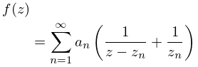
Mittag-Leffler’s Expansion
If and are sequences such that () and is convergent, then
| 1.10.25 | |||
is analytic in , except for simple poles at of residue .
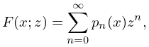
§1.10(xi) Generating Functions
Let have a converging power series expansion of the form
| 1.10.26 | |||
| . | |||
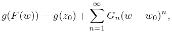
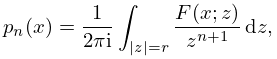
The radius of convergence might depend on . Then is the generating function for the functions , which will automatically have an integral representation
| 1.10.27 | |||
| ; | |||
compare (1.10.7). Often Darboux’s method can be used to study the behavior of as . Compare §2.10(iv).
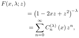
Example
Ultraspherical polynomials have generating function
| 1.10.28 | |||
| . | |||
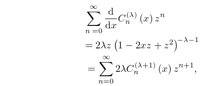
Many properties are a direct consequence of this representation: Taking the -derivative gives us
| 1.10.29 | |||
and hence , that is (18.9.19). The recurrence relation for in §18.9(i) follows from , and the contour integral representation for in §18.10(iii) is just (1.10.27).
