§3.11 Approximation Techniques
Contents
- §3.11(i) Minimax Polynomial Approximations
- §3.11(ii) Chebyshev-Series Expansions
- §3.11(iii) Minimax Rational Approximations
- §3.11(iv) Padé Approximations
- §3.11(v) Least Squares Approximations
- §3.11(vi) Splines
§3.11(i) Minimax Polynomial Approximations
Let be continuous on a closed interval . Then there exists a unique th degree polynomial , called the minimax (or best uniform) polynomial approximation to on , that minimizes , where .
A sufficient condition for to be the minimax polynomial is that attains its maximum at distinct points in and changes sign at these consecutive maxima.
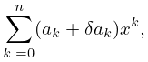
If we have a sufficiently close approximation
| 3.11.1 | |||
to , then the coefficients can be computed iteratively. Assume that is continuous on and let , , and be the zeros of in arranged so that
| 3.11.2 | |||
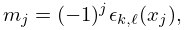
Also, let
| 3.11.3 | |||
| . | |||
(Thus the are approximations to , where is the maximum value of on .)
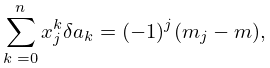
Then (in general) a better approximation to is given by
| 3.11.4 | |||
where
| 3.11.5 | |||
| . | |||
This is a set of equations for the unknowns and .
The iterative process converges locally and quadratically (§3.8(i)).
A method for obtaining a sufficiently accurate first approximation is described in the next subsection.
§3.11(ii) Chebyshev-Series Expansions
The Chebyshev polynomials are given by
| 3.11.6 | |||
| . | |||
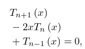
They satisfy the recurrence relation
| 3.11.7 | |||
| , | |||
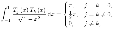
with initial values , . They enjoy an orthogonal property with respect to integrals:
| 3.11.8 | |||
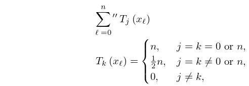
as well as an orthogonal property with respect to sums, as follows. When and , ,
| 3.11.9 | |||
where and the double prime means that the first and last terms are to be halved.
For these and further properties of Chebyshev polynomials, see Chapter 18, Gil et al. (2007a, Chapter 3), and Mason and Handscomb (2003).
Chebyshev Expansions
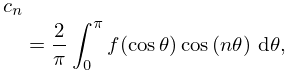
If is continuously differentiable on , then with
| 3.11.10 | |||
| , | |||
the expansion
| 3.11.11 | |||
| , | |||
converges uniformly. Here the single prime on the summation symbol means that the first term is to be halved. In fact, (3.11.11) is the Fourier-series expansion of ; compare (3.11.6) and §1.8(i).
Furthermore, if , then the convergence of (3.11.11) is usually very rapid; compare (1.8.7) with arbitrary.
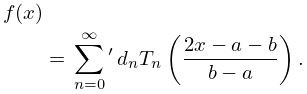
For general intervals we rescale:
| 3.11.12 | |||
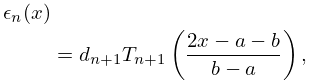
Because the series (3.11.12) converges rapidly we obtain a very good first approximation to the minimax polynomial for if we truncate (3.11.12) at its th term. This is because in the notation of §3.11(i)
| 3.11.13 | |||
approximately, and the right-hand side enjoys exactly those properties concerning its maxima and minima that are required for the minimax approximation; compare Figure 18.4.3.
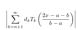
More precisely, it is known that for the interval , the ratio of the maximum value of the remainder
| 3.11.14 | |||
to the maximum error of the minimax polynomial is bounded by , where is the th Lebesgue constant for Fourier series; see §1.8(i). Since , is a monotonically increasing function of , and (for example) , this means that in practice the gain in replacing a truncated Chebyshev-series expansion by the corresponding minimax polynomial approximation is hardly worthwhile. Moreover, the set of minimax approximations requires the calculation and storage of coefficients, whereas the corresponding set of Chebyshev-series approximations requires only coefficients.
Calculation of Chebyshev Coefficients
The in (3.11.11) can be calculated from (3.11.10), but in general it is more efficient to make use of the orthogonal property (3.11.9). Also, in cases where satisfies a linear ordinary differential equation with polynomial coefficients, the expansion (3.11.11) can be substituted in the differential equation to yield a recurrence relation satisfied by the .
Summation of Chebyshev Series: Clenshaw’s Algorithm
For the expansion (3.11.11), numerical values of the Chebyshev polynomials can be generated by application of the recurrence relation (3.11.7). A more efficient procedure is as follows. Let be the last term retained in the truncated series. Beginning with , , we apply
| 3.11.15 | |||
| . | |||
Then the sum of the truncated expansion equals . For error analysis and modifications of Clenshaw’s algorithm, see Oliver (1977).
Complex Variables
If is replaced by a complex variable and is analytic, then the expansion (3.11.11) converges within an ellipse. However, in general (3.11.11) affords no advantage in for numerical purposes compared with the Maclaurin expansion of .
For further details on Chebyshev-series expansions in the complex plane, see Mason and Handscomb (2003, §5.10).
§3.11(iii) Minimax Rational Approximations
Let be continuous on a closed interval and be a continuous nonvanishing function on : is called a weight function. Then the minimax (or best uniform) rational approximation
| 3.11.16 | |||
of type to on minimizes the maximum value of on , where
| 3.11.17 | |||
The theory of polynomial minimax approximation given in §3.11(i) can be extended to the case when is replaced by a rational function . There exists a unique solution of this minimax problem and there are at least values , , such that , where
| 3.11.18 | |||
| , | |||
and is the maximum of on .
A collection of minimax rational approximations to elementary and special functions can be found in Hart et al. (1968).
A widely implemented and used algorithm for calculating the coefficients and in (3.11.16) is Remez’s second algorithm. See Remez (1957), Werner et al. (1967), and Johnson and Blair (1973).
Example
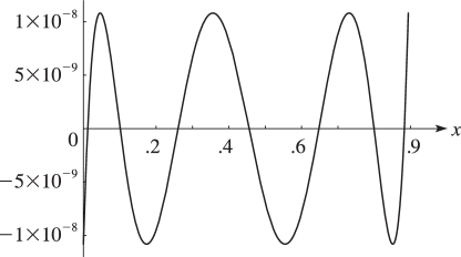
With and 14-digit computation, we obtain the following rational approximation of type to the Bessel function (§10.2(ii)) on the interval , where is the first positive zero of :
| 3.11.19 | |||
with coefficients given in Table 3.11.1.
| 0 | 0.99999 99891 7854 | |
|---|---|---|
| 1 | 0.34038 93820 9347 | 0.34039 05233 8838 |
| 2 | 0.18915 48376 3222 | 0.06086 50162 9812 |
| 3 | 0.06658 31942 0166 | 0.01864 47680 9090 |
The error curve is shown in Figure 3.11.1.
§3.11(iv) Padé Approximations
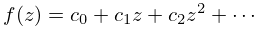
Let
| 3.11.20 | |||
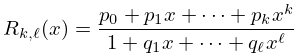
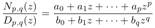
be a formal power series. The rational function
| 3.11.21 | |||
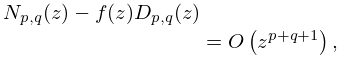
is called a Padé approximant at zero of if
| 3.11.22 | |||
| . | |||
It is denoted by . Thus if , then the Maclaurin expansion of (3.11.21) agrees with (3.11.20) up to, and including, the term in .
The requirement (3.11.22) implies
| 3.11.23 | ||||
where if . With , the last equations give as the solution of a system of linear equations. The first equations then yield .
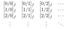
The array of Padé approximants
| 3.11.24 | |||
is called a Padé table. Approximants with the same denominator degree are located in the same column of the table.
For convergence results for Padé approximants, and the connection with continued fractions and Gaussian quadrature, see Baker and Graves-Morris (1996, §4.7).
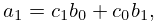
The Padé approximants can be computed by Wynn’s cross rule. Any five approximants arranged in the Padé table as
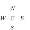
satisfy
| 3.11.25 | |||
Starting with the first column , , and initializing the preceding column by , , we can compute the lower triangular part of the table via (3.11.25). Similarly, the upper triangular part follows from the first row , , by initializing , .
For the recursive computation of by Wynn’s epsilon algorithm, see (3.9.11) and the subsequent text.
Laplace Transform Inversion
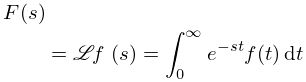
Numerical inversion of the Laplace transform (§1.14(iii))
| 3.11.26 | |||
requires to be obtained from numerical values of . A general procedure is to approximate by a rational function (vanishing at infinity) and then approximate by . When has an explicit power-series expansion a possible choice of is a Padé approximation to . See Luke (1969b, §16.4) for several examples involving special functions.
§3.11(v) Least Squares Approximations
Suppose a function is approximated by the polynomial
| 3.11.27 | |||
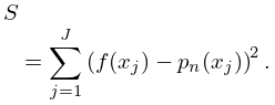
that minimizes
| 3.11.28 | |||
Here , , is a given set of distinct real points and . From the equations , , we derive the normal equations
| 3.11.29 | |||
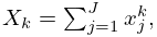
where
| 3.11.30 | ||||
(3.11.29) is a system of linear equations for the coefficients . The matrix is symmetric and positive definite, but the system is ill-conditioned when is large because the lower rows of the matrix are approximately proportional to one another. If , then is the Lagrange interpolation polynomial for the set (§3.3(i)).
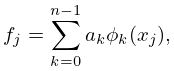
More generally, let be approximated by a linear combination
| 3.11.31 | |||
of given functions , , that minimizes
| 3.11.32 | |||
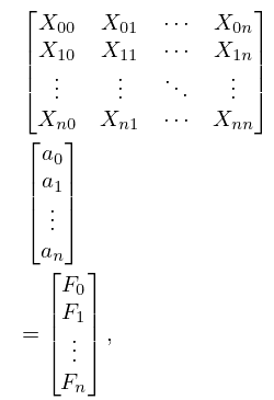
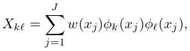
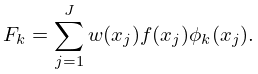
being a given positive weight function, and again . Then (3.11.29) is replaced by
| 3.11.33 | |||
with
| 3.11.34 | |||
and
| 3.11.35 | |||
Since , the matrix is again symmetric.
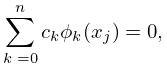
If the functions are linearly independent on the set , that is, the only solution of the system of equations
| 3.11.36 | |||
| , | |||
is , then the approximation is determined uniquely.
Now suppose that when , that is, the functions are orthogonal with respect to weighted summation on the discrete set . Then the system (3.11.33) is diagonal and hence well-conditioned.
A set of functions that is linearly independent on the set (compare (3.11.36)) can always be orthogonalized in the sense given in the preceding paragraph by the Gram–Schmidt procedure; see Gautschi (1997a).
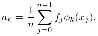
Example. The Discrete Fourier Transform
We take complex exponentials , , and approximate by the linear combination (3.11.31). The functions are orthogonal on the set , , with respect to the weight function , in the sense that
| 3.11.37 | |||
| , | |||
being Kronecker’s symbol and the bar denoting complex conjugate. In consequence we can solve the system
| 3.11.38 | |||
| , | |||
and obtain
| 3.11.39 | |||
| . | |||
With this choice of and , the corresponding sum (3.11.32) vanishes.
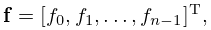
The pair of vectors
| 3.11.40 | ||||
is called a discrete Fourier transform pair.
The Fast Fourier Transform
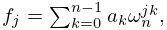
The direct computation of the discrete Fourier transform (3.11.38), that is, of
| 3.11.41 | ||||
| , | ||||
| , | ||||
requires approximately multiplications. The method of the fast Fourier transform (FFT) exploits the structure of the matrix with elements , . If , then can be factored into matrices, the rows of which contain only a few nonzero entries and the nonzero entries are equal apart from signs. In consequence of this structure the number of operations can be reduced to operations.
§3.11(vi) Splines
Splines are defined piecewise and usually by low-degree polynomials. Given distinct points in the real interval , with ()(), on each subinterval , , a low-degree polynomial is defined with coefficients determined by, for example, values and of a function and its derivative at the nodes and . The set of all the polynomials defines a function, the spline, on . By taking more derivatives into account, the smoothness of the spline will increase.
For splines based on Bernoulli and Euler polynomials, see §24.17(ii).
For many applications a spline function is a more adaptable approximating tool than the Lagrange interpolation polynomial involving a comparable number of parameters; see §3.3(i), where a single polynomial is used for interpolating on the complete interval . Multivariate functions can also be approximated in terms of multivariate polynomial splines. See de Boor (2001), Chui (1988), and Schumaker (1981) for further information.
In computer graphics a special type of spline is used which produces a Bézier curve. A cubic Bézier curve is defined by four points. Two are endpoints: and ; the other points and are control points. The slope of the curve at is tangent to the line between and ; similarly the slope at is tangent to the line between and . The curve is described by and , which are cubic polynomials with . A complete spline results by composing several Bézier curves. A special applications area of Bézier curves is mathematical typography and the design of type fonts. See Knuth (1986, pp. 116-136).
