Chebyshev polynomials
(0.005 seconds)
1—10 of 47 matching pages
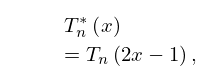
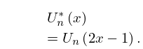
1: 18.3 Definitions
§18.3 Definitions
… ►| Name | Constraints | ||||||
|---|---|---|---|---|---|---|---|
| … | |||||||
| Chebyshev of second kind | |||||||
| … | |||||||
| Shifted Chebyshev of second kind | |||||||
| … | |||||||
2: 18.41 Tables
…
►For () see §14.33.
►Abramowitz and Stegun (1964, Tables 22.4, 22.6, 22.11, and 22.13) tabulates , , , and for .
The ranges of are for and , and for and .
…
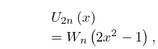
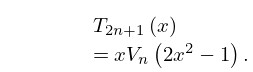
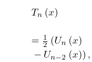
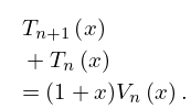
3: 18.7 Interrelations and Limit Relations
4: 18.9 Recurrence Relations and Derivatives
…
►
…
►
18.9.9
…
►
18.9.12
►Identities similar to (18.9.11) and (18.9.12) involving and can be obtained using rows 4 and 7 in Table 18.6.1.
…
5: 18.1 Notation
…
►
►
…
►Nor do we consider the shifted Jacobi polynomials:
…
►
►
…
Chebyshev of first, second, third, and fourth kinds: , , , .
Shifted Chebyshev of first and second kinds: , .
6: 18.6 Symmetry, Special Values, and Limits to Monomials
7: 18.5 Explicit Representations
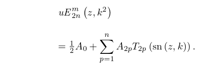
8: 29.15 Fourier Series and Chebyshev Series
…
►
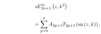
§29.15(ii) Chebyshev Series
►The Chebyshev polynomial of the first kind (§18.3) satisfies . … ►
29.15.43
…
►Using also , with denoting the Chebyshev polynomial of the second kind (§18.3), we obtain
►
29.15.44
…
9: 3.11 Approximation Techniques
…
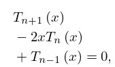
►The Chebyshev polynomials
are given by
…
►
3.11.7
,
►with initial values , .
…
►For the expansion (3.11.11), numerical values of the Chebyshev polynomials
can be generated by application of the recurrence relation (3.11.7).
…Let be the last term retained in the truncated series.
…
