singularity parameter

SearchAdvancedHelp

(0.001 seconds)

11—20 of 61 matching pages

11: 2.8 Differential Equations with a Parameter

… ►The form of the asymptotic expansion depends on the nature of the transition points in $𝐃$, that is, points at which $f(z)$ has a zero or singularity. …

12: 28.2 Definitions and Basic Properties

… ►

28.2.2 $$\zeta (1-\zeta )w^{\prime \prime }+\frac{1}{2}(1-2\zeta )w^{\prime }+\frac{1}{4}(a-2q(1-2\zeta ))w=0.$$

ⓘ

Symbols:

$q=h^2$: parameter, $a$: parameter, $w(z)$: Mathieu’s equation solution and $\zeta$: change of variable

Permalink:

http://dlmf.nist.gov/28.2.E2

Encodings:

pMML, png, TeX

See also:

Annotations for §28.2(i), §28.2 and Ch.28

…

13: 31.12 Confluent Forms of Heun’s Equation

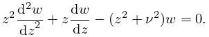
… ►Confluent forms of Heun’s differential equation (31.2.1) arise when two or more of the regular singularities merge to form an irregular singularity. … ►This has regular singularities at $z=0$ and $1$, and an irregular singularity of rank 1 at $z=\mathrm{\infty }$. … ►This has irregular singularities at $z=0$ and $\mathrm{\infty }$, each of rank $1$. … ►This has a regular singularity at $z=0$, and an irregular singularity at $\mathrm{\infty }$ of rank $2$. … ►This has one singularity, an irregular singularity of rank $3$ at $z=\mathrm{\infty }$. …

14: 33.14 Definitions and Basic Properties

… ►

§33.14(i) Coulomb Wave Equation

… ►

33.14.1 $$\frac{d^{2}w}{{dr}^2}+\left(ϵ+\frac{2}{r}-\frac{\mathrm{\ell }(\mathrm{\ell }+1)}{r^2}\right)w=0,$$

ⓘ

Symbols:

$\frac{df}{dx}$: derivative of $f$ with respect to $x$ , $\mathrm{\ell }$: nonnegative integer, $r$: real variable and $ϵ$: real parameter

Referenced by:

§33.23(iii)

Permalink:

http://dlmf.nist.gov/33.14.E1

Encodings:

pMML, png, TeX

See also:

Annotations for §33.14(i), §33.14 and Ch.33

… ►Again, there is a regular singularity at $r=0$ with indices $\mathrm{\ell }+1$ and $-\mathrm{\ell }$, and an irregular singularity of rank 1 at $r=\mathrm{\infty }$. … ►

33.14.3 $$r_{\mathrm{tp}}(ϵ,\mathrm{\ell })=\left(\sqrt{1+ϵ\mathrm{\ell }(\mathrm{\ell }+1)}-1\right)/ϵ;$$

ⓘ

Defines:

$r_{\mathrm{tp}}(ϵ,\mathrm{\ell })$: outer turning point for Coulomb functions

Symbols:

$\mathrm{\ell }$: nonnegative integer and $ϵ$: real parameter

Permalink:

http://dlmf.nist.gov/33.14.E3

Encodings:

pMML, png, TeX

See also:

Annotations for §33.14(i), §33.14 and Ch.33

… ►

33.14.11 $$A(ϵ,\mathrm{\ell })=\prod _{k=0}^{\mathrm{\ell }}(1+ϵk^2).$$

ⓘ

Defines:

$A(ϵ,\mathrm{\ell })$: function (locally)

Symbols:

$k$: nonnegative integer, $\mathrm{\ell }$: nonnegative integer and $ϵ$: real parameter

Referenced by:

§33.14(iv), §33.16(ii), §33.16(iii), §33.19, §33.20(iii)

Permalink:

http://dlmf.nist.gov/33.14.E11

Encodings:

pMML, png, TeX

See also:

Annotations for §33.14(iv), §33.14 and Ch.33

…

15: 29.2 Differential Equations

… ►where $k$ and $\nu$ are real parameters such that and $\nu \ge -\frac{1}{2}$. …This equation has regular singularities at the points $2pK+(2q+1)\mathrm{i}{K}^{\prime }$, where $p,q\in \mathbb{Z}$, and $K$, $K^{\prime }$ are the complete elliptic integrals of the first kind with moduli $k$, $k^{\prime }(={(1-k^2)}^{1/2})$, respectively; see §19.2(ii). In general, at each singularity each solution of (29.2.1) has a branch point (§2.7(i)). … ►

Figure 29.2.1: $z$-plane: singularities $\times$ $\times$ $\times$ of Lamé’s equation.

… ►

29.2.7 $$g=(e_1-e_3)h+\nu (\nu +1)e_3,$$

ⓘ

Defines:

$g$ (locally)

Symbols:

$h$: real parameter, $\nu$: real parameter and $e_j$: constants

Permalink:

http://dlmf.nist.gov/29.2.E7

Encodings:

pMML, png, TeX

See also:

Annotations for §29.2(ii), §29.2 and Ch.29

…

16: 31.5 Solutions Analytic at Three Singularities: Heun Polynomials

§31.5 Solutions Analytic at Three Singularities: Heun Polynomials

… ►

31.5.1

ⓘ

Symbols:

$\gamma$: real or complex parameter, $n$: nonnegative integer, $a$: complex parameter, $P_j$: coefficient, $Q_j$: coefficient and $R_j$: coefficient

Permalink:

http://dlmf.nist.gov/31.5.E1

Encodings:

pMML, png, TeX

See also:

Annotations for §31.5 and Ch.31

… ►

31.5.2 $${\mathrm{𝐻𝑝}}_{n,m}(a,q_{n,m};-n,\beta ,\gamma ,\delta ;z)=H\mathrm{\ell }(a,q_{n,m};-n,\beta ,\gamma ,\delta ;z)$$

ⓘ

Defines:

${\mathrm{𝐻𝑝}}_{n,m}(a,q_{n,m};-n,\beta ,\gamma ,\delta ;z)$: Heun polynomials

Symbols:

$H\mathrm{\ell }(a,q;\alpha ,\beta ,\gamma ,\delta ;z)$: Heun functions, $z$: complex variable, $\gamma$: real or complex parameter, $\delta$: real or complex parameter, $m$: nonnegative integer, $n$: nonnegative integer, $a$: complex parameter, $q$: real or complex parameter and $\beta$: real or complex parameter

Permalink:

http://dlmf.nist.gov/31.5.E2

Encodings:

pMML, png, TeX

See also:

Annotations for §31.5 and Ch.31

►is a polynomial of degree $n$, and hence a solution of (31.2.1) that is analytic at all three finite singularities $0,1,a$. …

17: 10.25 Definitions

… ►

10.25.1 $$z^2\frac{d^{2}w}{{dz}^2}+z\frac{dw}{dz}-(z^2+{\nu }^2)w=0.$$

ⓘ

Symbols:

$\frac{df}{dx}$: derivative of $f$ with respect to $x$ , $z$: complex variable and $\nu$: complex parameter

A&S Ref:

9.6.1

Referenced by:

§10.25(ii), §10.25(iii), §10.27, §10.45, §10.74(ii)

Permalink:

http://dlmf.nist.gov/10.25.E1

Encodings:

pMML, png, TeX

See also:

Annotations for §10.25(i), §10.25 and Ch.10

►This equation is obtained from Bessel’s equation (10.2.1) on replacing $z$ by $\pm \mathrm{i}z$, and it has the same kinds of singularities. … … ►

10.25.2 $$I_{\nu }\left(z\right)={(\frac{1}{2}z)}^{\nu }\sum _{k=0}^{\mathrm{\infty }}\frac{{(\frac{1}{4}{z}^2)}^k}{k!\mathrm{\Gamma }\left(\nu +k+1\right)}.$$

ⓘ

Defines:

$I_{\nu }\left(z\right)$: modified Bessel function of the first kind

Symbols:

$\mathrm{\Gamma }\left(z\right)$: gamma function, $!$: factorial (as in $n!$), $k$: nonnegative integer, $z$: complex variable and $\nu$: complex parameter

A&S Ref:

9.6.10

Referenced by:

§10.30(i), §10.31, §10.38, §10.45, §10.46, §10.53, §8.6(i)

Permalink:

http://dlmf.nist.gov/10.25.E2

Encodings:

pMML, png, TeX

See also:

Annotations for §10.25(ii), §10.25 and Ch.10

… ►

10.25.3 $$K_{\nu }\left(z\right)\sim \sqrt{\pi /(2z)}{\mathrm{e}}^{-z},$$

ⓘ

Defines:

$K_{\nu }\left(z\right)$: modified Bessel function of the second kind

Symbols:

$\sim$: asymptotic equality, $\pi$: the ratio of the circumference of a circle to its diameter, $\mathrm{e}$: base of natural logarithm, $z$: complex variable and $\nu$: complex parameter

Referenced by:

§10.25(ii), §10.25(iii), §10.30(ii)

Permalink:

http://dlmf.nist.gov/10.25.E3

Encodings:

pMML, png, TeX

See also:

Annotations for §10.25(ii), §10.25 and Ch.10

…

18: 15.11 Riemann’s Differential Equation

… ►

§15.11(i) Equations with Three Singularities

►The importance of (15.10.1) is that any homogeneous linear differential equation of the second order with at most three distinct singularities, all regular, in the extended plane can be transformed into (15.10.1). … ►

15.11.2 $$a_1+a_2+b_1+b_2+c_1+c_2=1.$$

ⓘ

Symbols:

$a$: real or complex parameter, $b$: real or complex parameter and $c$: real or complex parameter

Permalink:

http://dlmf.nist.gov/15.11.E2

Encodings:

pMML, png, TeX

See also:

Annotations for §15.11(i), §15.11 and Ch.15

… ►Cases in which there are fewer than three singularities are included automatically by allowing the choice $\{0,1\}$ for exponent pairs. … ►The reduction of a general homogeneous linear differential equation of the second order with at most three regular singularities to the hypergeometric differential equation is given by …

19: 31.6 Path-Multiplicative Solutions

… ►

31.6.1 $$(s_1,s_2){\mathrm{𝐻𝑓}}_m^{\nu }(a,q_m;\alpha ,\beta ,\gamma ,\delta ;z),$$ $m=0,1,2,\mathrm{\dots }$,

ⓘ

Symbols:

$(s_1,s_2){\mathrm{𝐻𝑓}}_m(a,q_m;\alpha ,\beta ,\gamma ,\delta ;z)$: Heun functions, $z$: complex variable, $\gamma$: real or complex parameter, $\delta$: real or complex parameter, $\nu$: real or complex parameter, $m$: nonnegative integer, $a$: complex parameter, $q$: real or complex parameter, $\alpha$: real or complex parameter, $\beta$: real or complex parameter and $s_j$: parameters

Permalink:

http://dlmf.nist.gov/31.6.E1

Encodings:

pMML, png, TeX

See also:

Annotations for §31.6 and Ch.31

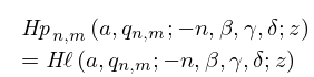
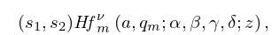
… ►This denotes a set of solutions of (31.2.1) with the property that if we pass around a simple closed contour in the $z$-plane that encircles $s_1$ and $s_2$ once in the positive sense, but not the remaining finite singularity, then the solution is multiplied by a constant factor ${\mathrm{e}}^{2\nu \pi \mathrm{i}}$. …

20: 33.2 Definitions and Basic Properties

… ►

§33.2(i) Coulomb Wave Equation

►

33.2.1 $$\frac{d^{2}w}{{d\rho }^2}+\left(1-\frac{2\eta }{\rho }-\frac{\mathrm{\ell }(\mathrm{\ell }+1)}{{\rho }^2}\right)w=0,$$ $\mathrm{\ell }=0,1,2,\mathrm{\dots }$.

ⓘ

Symbols:

$\frac{df}{dx}$: derivative of $f$ with respect to $x$ , $\mathrm{\ell }$: nonnegative integer, $\rho$: nonnegative real variable and $\eta$: real parameter

Referenced by:

§33.12(ii), §33.14(i), §33.22(iv), §33.23(iii)

Permalink:

http://dlmf.nist.gov/33.2.E1

Encodings:

pMML, png, TeX

See also:

Annotations for §33.2(i), §33.2 and Ch.33

►This differential equation has a regular singularity at $\rho =0$ with indices $\mathrm{\ell }+1$ and $-\mathrm{\ell }$, and an irregular singularity of rank 1 at $\rho =\mathrm{\infty }$ (§§2.7(i), 2.7(ii)). … ►

33.2.2 $${\rho }_{\mathrm{tp}}(\eta ,\mathrm{\ell })=\eta +{({\eta }^2+\mathrm{\ell }(\mathrm{\ell }+1))}^{1/2}.$$

ⓘ

Defines:

${\rho }_{\mathrm{tp}}(\eta ,\mathrm{\ell })$: outer turning point for Coulomb radial functions

Symbols:

$\mathrm{\ell }$: nonnegative integer and $\eta$: real parameter

Referenced by:

§33.12(i), §33.14(i)

Permalink:

http://dlmf.nist.gov/33.2.E2

Encodings:

pMML, png, TeX

See also:

Annotations for §33.2(i), §33.2 and Ch.33

… ►

33.2.10 $${\sigma }_{\mathrm{\ell }}\left(\eta \right)=\mathrm{ph}\mathrm{\Gamma }\left(\mathrm{\ell }+1+\mathrm{i}\eta \right),$$

ⓘ

Defines:

${\sigma }_{\mathrm{\ell }}\left(\eta \right)$: Coulomb phase shift

Symbols:

$\mathrm{\Gamma }\left(z\right)$: gamma function, $\mathrm{i}$: imaginary unit, $\mathrm{ph}$: phase, $\mathrm{\ell }$: nonnegative integer and $\eta$: real parameter

A&S Ref:

14.5.6

Referenced by:

§33.10(ii), §33.10(iii), §33.13, §33.2(iii), §33.25, §5.20

Permalink:

http://dlmf.nist.gov/33.2.E10

Encodings:

pMML, png, TeX

See also:

Annotations for §33.2(iii), §33.2 and Ch.33

…