scaling laws

SearchAdvancedHelp

(0.001 seconds)

11—20 of 72 matching pages

11: 15.1 Special Notation

… ►

15.1.2 $$\frac{F(a,b;c;z)}{\mathrm{\Gamma }\left(c\right)}=𝐅(a,b;c;z)=𝐅(\genfrac{}{}{0pt}{}{a,b}{c};z)={}_2{}^{}𝐅_1^{}(a,b;c;z),$$

ⓘ

Symbols:

$\mathrm{\Gamma }\left(z\right)$: gamma function, $F(a,b;c;z)$ or $F(\genfrac{}{}{0pt}{}{a,b}{c};z)$: $={}_2{}^{}F_1^{}(a,b;c;z)$ Gauss’ hypergeometric function, ${}_p{}^{}𝐅_q^{}(𝐚;𝐛;z)$ or ${}_p{}^{}𝐅_q^{}(\genfrac{}{}{0pt}{}{𝐚}{𝐛};z)$: scaled (or Olver’s) generalized hypergeometric function, $𝐅(a,b;c;z)$ or $𝐅(\genfrac{}{}{0pt}{}{a,b}{c};z)$: $={}_2{}^{}𝐅_1^{}(a,b;c;z)$ Olver’s hypergeometric function, $z$: complex variable, $a$: real or complex parameter, $b$: real or complex parameter and $c$: real or complex parameter

Permalink:

http://dlmf.nist.gov/15.1.E2

Encodings:

pMML, png, TeX

See also:

Annotations for §15.1 and Ch.15

…

12: 15.2 Definitions and Analytical Properties

… ►Except where indicated otherwise principal branches of $F(a,b;c;z)$ and $𝐅(a,b;c;z)$ are assumed throughout the DLMF. … ►The principal branch of $𝐅(a,b;c;z)$ is an entire function of $a$, $b$, and $c$. …As a multivalued function of $z$, $𝐅(a,b;c;z)$ is analytic everywhere except for possible branch points at $z=0$, $1$, and $\mathrm{\infty }$. … ►(Both interpretations give solutions of the hypergeometric differential equation (15.10.1), as does $𝐅(a,b;c;z)$, which is analytic at $c=0,-1,-2,\mathrm{\dots }$.) ►For comparison of $F(a,b;c;z)$ and $𝐅(a,b;c;z)$, with the former using the limit interpretation (15.2.5), see Figures 15.3.6 and 15.3.7. …

13: 15.14 Integrals

… ►

15.14.1 $${\int }_0^{\mathrm{\infty }}{x}^{s-1}𝐅(\genfrac{}{}{0pt}{}{a,b}{c};-x)dx=\frac{\mathrm{\Gamma }\left(s\right)\mathrm{\Gamma }\left(a-s\right)\mathrm{\Gamma }\left(b-s\right)}{\mathrm{\Gamma }\left(a\right)\mathrm{\Gamma }\left(b\right)\mathrm{\Gamma }\left(c-s\right)},$$ $\min (\mathrm{\Re }a,\mathrm{\Re }b)>\mathrm{\Re }s>0$.

ⓘ

Symbols:

$\mathrm{\Gamma }\left(z\right)$: gamma function, $dx$: differential of $x$ , $\int$: integral, $\mathrm{\Re }$: real part, $𝐅(a,b;c;z)$ or $𝐅(\genfrac{}{}{0pt}{}{a,b}{c};z)$: $={}_2{}^{}𝐅_1^{}(a,b;c;z)$ Olver’s hypergeometric function, $x$: real variable, $s$: nonnegative integer, $a$: real or complex parameter, $b$: real or complex parameter and $c$: real or complex parameter

Keywords:

Mellin transform

Referenced by:

§15.14

Permalink:

http://dlmf.nist.gov/15.14.E1

Encodings:

pMML, png, TeX

See also:

Annotations for §15.14 and Ch.15

…

14: 30.15 Signal Analysis

… ►

§30.15(i) Scaled Spheroidal Wave Functions

… ►

§30.15(ii) Integral Equation

… ► ►

§30.15(iv) Orthogonality

… ►

§30.15(v) Extremal Properties

…

15: 36.5 Stokes Sets

… ►For $z\ne 0$, the Stokes set is expressed in terms of scaled coordinates … ►

36.5.7 $$X=\frac{9}{20}+20u^4-\frac{Y^2}{20u^2}+6u^2\mathrm{sign}\left(z\right),$$

ⓘ

Symbols:

$\mathrm{sign}x$: sign of, $z$: real parameter, $X$: scaled coordinate and $Y$: scaled coordinate

Permalink:

http://dlmf.nist.gov/36.5.E7

Encodings:

pMML, png, TeX

See also:

Annotations for §36.5(ii), §36.5(ii), §36.5 and Ch.36

… ►

36.5.10 $$160u^6+40u^4=Y^2.$$

ⓘ

Symbols:

$Y$: scaled coordinate

Permalink:

http://dlmf.nist.gov/36.5.E10

Encodings:

pMML, png, TeX

See also:

Annotations for §36.5(ii), §36.5(ii), §36.5 and Ch.36

… ►

36.5.17 $$Y_{\mathrm{S}}(X)=Y(u,|X|),$$

ⓘ

Symbols:

$X$: scaled coordinate

Permalink:

http://dlmf.nist.gov/36.5.E17

Encodings:

pMML, png, TeX

See also:

Annotations for §36.5(iii), §36.5(iii), §36.5 and Ch.36

… ►

36.5.18 $$f(u,X)=f(-u+\frac{1}{3},X),$$

ⓘ

Symbols:

$X$: scaled coordinate

Permalink:

http://dlmf.nist.gov/36.5.E18

Encodings:

pMML, png, TeX

See also:

Annotations for §36.5(iii), §36.5(iii), §36.5 and Ch.36

…

16: 5.11 Asymptotic Expansions

… ►

5.11.3 $$\mathrm{\Gamma }\left(z\right)={\mathrm{e}}^{-z}{z}^z{\left(\frac{2\pi }{z}\right)}^{1/2}{\mathrm{\Gamma }}^{\ast }\left(z\right)\sim {\mathrm{e}}^{-z}{z}^z{\left(\frac{2\pi }{z}\right)}^{1/2}\sum _{k=0}^{\mathrm{\infty }}\frac{g_k}{z^k},$$

ⓘ

Defines:

${\mathrm{\Gamma }}^{\ast }\left(z\right)$: scaled gamma function

Symbols:

$\mathrm{\Gamma }\left(z\right)$: gamma function, $\sim$: Poincaré asymptotic expansion, $\pi$: the ratio of the circumference of a circle to its diameter, $\mathrm{e}$: base of natural logarithm, $k$: nonnegative integer, $z$: complex variable and $g_k$: coefficients

A&S Ref:

6.1.37

Referenced by:

§10.19(i), §13.8(iv), §5.11(i), §5.11(i), §5.11(i), §5.11(ii), §5.11(ii), §5.21, §5.9(i), §8.11(ii), §8.12, (8.18.13), (8.18.13), §8.18(ii), §8.18(ii), Erratum (V1.1.7) for Additions, Erratum (V1.1.8) for Rearrangement

Permalink:

http://dlmf.nist.gov/5.11.E3

Encodings:

pMML, png, TeX

Addition (effective with 1.1.7):

The definition of the scaled gamma function ${\mathrm{\Gamma }}^{\ast }\left(z\right)$ was inserted after the first equals sign.

Changes (effective with 1.0.11):

An unnecessary bracket around the sum was removed.

See also:

Annotations for §5.11(i), §5.11 and Ch.5

… ►The scaled gamma function ${\mathrm{\Gamma }}^{\ast }\left(z\right)$ is defined in (5.11.3) and its main property is ${\mathrm{\Gamma }}^{\ast }\left(z\right)\sim 1$ as $z\to \mathrm{\infty }$ in the sector $|\mathrm{ph}z|\le \pi -\delta$. …

17: 8.18 Asymptotic Expansions of $I_x(a,b)$

… ►

General Case

►For the scaled gamma function ${\mathrm{\Gamma }}^{\ast }\left(z\right)$ see (5.11.3). … ►

8.18.14 $$I_x(a,b)\sim Q(b,a\zeta )-\frac{{(2\pi b)}^{-1/2}}{{\mathrm{\Gamma }}^{\ast }\left(b\right)}{\left(\frac{x}{x_0}\right)}^a{\left(\frac{1-x}{1-x_0}\right)}^b\sum _{k=0}^{\mathrm{\infty }}\frac{h_k(\zeta ,\mu )}{a^k},$$

ⓘ

Symbols:

$I_x(a,b)$: incomplete beta function, $\sim$: Poincaré asymptotic expansion, $\pi$: the ratio of the circumference of a circle to its diameter, $Q(a,z)$: normalized incomplete gamma function, ${\mathrm{\Gamma }}^{\ast }\left(z\right)$: scaled gamma function, $k$: nonnegative integer, $a$: parameter, $b$: parameter, $x$: variable, $\mu$ , $\zeta$: variable and $h_k(\zeta ,\mu )$: coefficients

Permalink:

http://dlmf.nist.gov/8.18.E14

Encodings:

pMML, png, TeX

See also:

Annotations for §8.18(ii), §8.18(ii), §8.18 and Ch.8

…

18: 21.4 Graphics

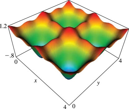
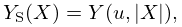
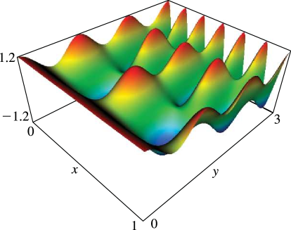
… ►Figure 21.4.1 provides surfaces of the scaled Riemann theta function $\widehat{\theta }\left(𝐳\right|𝛀)$, with … ►For the scaled Riemann theta functions depicted in Figures 21.4.2–21.4.5 … ►

►

►

Figure 21.4.4: A real-valued scaled Riemann theta function: $\widehat{\theta }\left(\mathrm{i}x,\mathrm{i}y\right|{𝛀}_1)$, $0\le x\le 4$, $0\le y\le 4$. … Magnify 3D Help

►

►

►

Figure 21.4.5: The real part of a genus 3 scaled Riemann theta function: $\mathrm{\Re }\widehat{\theta }\left(x+\mathrm{i}y,0,0\right|{𝛀}_2)$, $0\le x\le 1$, $0\le y\le 3$. … Magnify 3D Help

19: 23.20 Mathematical Applications

… ►In terms of $(x,y)$ the addition law can be expressed $(x,y)+o=(x,y)$, $(x,y)+(x,-y)=o$; otherwise $(x_1,y_1)+(x_2,y_2)=(x_3,y_3)$, where … ►

23.20.4

ⓘ

Symbols:

$m$: integer, $x$: real part of $z$ , $y$: imaginary part of $z$ , $a$: constant and $P$: points

Permalink:

http://dlmf.nist.gov/23.20.E4

Encodings:

pMML, png, TeX

See also:

Annotations for §23.20(ii), §23.20 and Ch.23

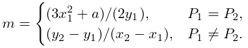
… ►The addition law states that to find the sum of two points, take the third intersection with $C$ of the chord joining them (or the tangent if they coincide); then its reflection in the $x$-axis gives the required sum. …

20: 5.9 Integral Representations

… ►

5.9.11_1 $${\mathrm{\Gamma }}^{\ast }\left(z\right)=1-\frac{1}{2\pi \mathrm{i}}{\int }_0^{\mathrm{\infty }}\frac{{\mathrm{e}}^{-2\pi t}{\mathrm{\Gamma }}^{\ast }\left(t{\mathrm{e}}^{\mathrm{i}\pi /2}\right)}{t+\mathrm{i}z}dt+\frac{1}{2\pi \mathrm{i}}{\int }_0^{\mathrm{\infty }}\frac{{\mathrm{e}}^{-2\pi t}{\mathrm{\Gamma }}^{\ast }\left(t{\mathrm{e}}^{-\mathrm{i}\pi /2}\right)}{t-\mathrm{i}z}dt,$$

ⓘ

Symbols:

$\pi$: the ratio of the circumference of a circle to its diameter, $dx$: differential of $x$ , $\mathrm{e}$: base of natural logarithm, $\mathrm{i}$: imaginary unit, $\int$: integral, ${\mathrm{\Gamma }}^{\ast }\left(z\right)$: scaled gamma function and $z$: complex variable

Source:

Boyd (1994, (2.16), p. 617)

Referenced by:

§5.9(i), Erratum (V1.1.7) for Additions

Permalink:

http://dlmf.nist.gov/5.9.E11_1

Encodings:

pMML, png, TeX

Addition (effective with 1.1.7):

This equation was added.

See also:

Annotations for §5.9(i), §5.9(i), §5.9 and Ch.5

►

5.9.11_2 $$\frac{1}{{\mathrm{\Gamma }}^{\ast }\left(z\right)}=1-\frac{1}{2\pi \mathrm{i}}{\int }_0^{\mathrm{\infty }}\frac{{\mathrm{e}}^{-2\pi t}{\mathrm{\Gamma }}^{\ast }\left(t{\mathrm{e}}^{\mathrm{i}\pi /2}\right)}{t-\mathrm{i}z}dt+\frac{1}{2\pi \mathrm{i}}{\int }_0^{\mathrm{\infty }}\frac{{\mathrm{e}}^{-2\pi t}{\mathrm{\Gamma }}^{\ast }\left(t{\mathrm{e}}^{-\mathrm{i}\pi /2}\right)}{t+\mathrm{i}z}dt,$$

ⓘ

Symbols:

$\pi$: the ratio of the circumference of a circle to its diameter, $dx$: differential of $x$ , $\mathrm{e}$: base of natural logarithm, $\mathrm{i}$: imaginary unit, $\int$: integral, ${\mathrm{\Gamma }}^{\ast }\left(z\right)$: scaled gamma function and $z$: complex variable

Source:

Boyd (1994, (4.2), p. 628)

Referenced by:

§5.9(i), Erratum (V1.1.7) for Additions

Permalink:

http://dlmf.nist.gov/5.9.E11_2

Encodings:

pMML, png, TeX

Addition (effective with 1.1.7):

This equation was added.

See also:

Annotations for §5.9(i), §5.9(i), §5.9 and Ch.5

►where , and the scaled gamma function ${\mathrm{\Gamma }}^{\ast }\left(z\right)$ is defined in (5.11.3). …