§23.20 Mathematical Applications
Contents
- §23.20(i) Conformal Mappings
- §23.20(ii) Elliptic Curves
- §23.20(iii) Factorization
- §23.20(iv) Modular and Quintic Equations
- §23.20(v) Modular Functions and Number Theory
§23.20(i) Conformal Mappings
Rectangular Lattice
The boundary of the rectangle , with vertices , , , , is mapped strictly monotonically by onto the real line with , , , , . There is a unique point such that . The interior of is mapped one-to-one onto the lower half-plane.
Rhombic Lattice
The two pairs of edges and of are each mapped strictly monotonically by onto the real line, with , , ; similarly for the other pair of edges. For each pair of edges there is a unique point such that .
The interior of the rectangle with vertices , , , is mapped two-to-one onto the lower half-plane. The interior of the rectangle with vertices , , , is mapped one-to-one onto the lower half-plane with a cut from to . The cut is the image of the edge from to and is not a line segment.
For examples of conformal mappings of the function , see Abramowitz and Stegun (1964, pp. 642–648, 654–655, and 659–60).
For conformal mappings via modular functions see Apostol (1990, §2.7).
§23.20(ii) Elliptic Curves
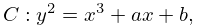
An algebraic curve that can be put either into the form
| 23.20.1 | |||
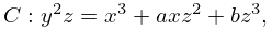
or equivalently, on replacing by and by (projective coordinates), into the form
| 23.20.2 | |||
is an example of an elliptic curve (§22.18(iv)). Here and are real or complex constants.
Points on the curve can be parametrized by , , where and : in this case we write . The curve is made into an abelian group (Macdonald (1968, Chapter 5)) by defining the zero element as the point at infinity, the negative of by , and generally on the curve iff the points , , are collinear. It follows from the addition formula (23.10.1) that the points , , have zero sum iff , so that addition of points on the curve corresponds to addition of parameters on the torus ; see McKean and Moll (1999, §§2.11, 2.14).
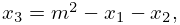
In terms of the addition law can be expressed , ; otherwise , where
| 23.20.3 | ||||
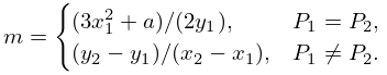
and
| 23.20.4 | |||
If , then intersects the plane in a curve that is connected if ; if , then the intersection has two components, one of which is a closed loop. These cases correspond to rhombic and rectangular lattices, respectively. The addition law states that to find the sum of two points, take the third intersection with of the chord joining them (or the tangent if they coincide); then its reflection in the -axis gives the required sum. The geometric nature of this construction is illustrated in McKean and Moll (1999, §2.14), Koblitz (1993, §§6, 7), and Silverman and Tate (1992, Chapter 1, §§3, 4): each of these references makes a connection with the addition theorem (23.10.1).
If , then by rescaling we may assume . Let denote the set of points on that are of finite order (that is, those points for which there exists a positive integer with ), and let be the sets of points with integer and rational coordinates, respectively. Then . Both are subgroups of , though may not be. always has the form (Mordell’s Theorem: Silverman and Tate (1992, Chapter 3, §5)); the determination of , the rank of , raises questions of great difficulty, many of which are still open. Both and are finite sets. must have one of the forms , or , or , . To determine , we make use of the fact that if then must be a divisor of ; hence there are only a finite number of possibilities for . Values of are then found as integer solutions of (in particular must be a divisor of ). The resulting points are then tested for finite order as follows. Given , calculate , , by doubling as above. If any of these quantities is zero, then the point has finite order. If any of , , is not an integer, then the point has infinite order. Otherwise observe any equalities between , , , , and their negatives. The order of a point (if finite and not already determined) can have only the values 3, 5, 6, 7, 9, 10, or 12, and so can be found from , , , , , , or . If none of these equalities hold, then has infinite order.
For extensive tables of elliptic curves see Cremona (1997, pp. 84–340).
§23.20(iii) Factorization
§23.20(iv) Modular and Quintic Equations
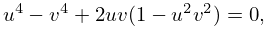
The modular equation of degree , prime, is an algebraic equation in and . For and with , , the modular equation is as follows:
| 23.20.5 | |||
| , | |||
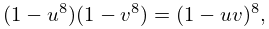
| 23.20.6 | |||
| , | |||
| 23.20.7 | |||
| , | |||
| 23.20.8 | |||
| . | |||
