pi

SearchAdvancedHelp

(0.001 seconds)

11—20 of 480 matching pages

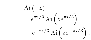
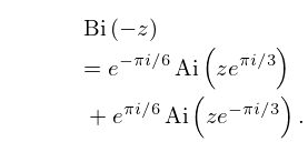
11: 6.4 Analytic Continuation

… ►

6.4.2 $$E_1\left(z{\mathrm{e}}^{2m\pi \mathrm{i}}\right)=E_1\left(z\right)-2m\pi \mathrm{i},$$ $m\in \mathbb{Z}$,

ⓘ

Symbols:

$\pi$: the ratio of the circumference of a circle to its diameter, $\in$: element of, $\mathrm{e}$: base of natural logarithm, $E_1\left(z\right)$: exponential integral, $\mathrm{i}$: imaginary unit, $\mathbb{Z}$: set of all integers and $z$: complex variable

Permalink:

http://dlmf.nist.gov/6.4.E2

Encodings:

pMML, png, TeX

See also:

Annotations for §6.4 and Ch.6

… ►

6.4.4 $$\mathrm{Ci}\left(z{\mathrm{e}}^{\pm \pi \mathrm{i}}\right)=\pm \pi \mathrm{i}+\mathrm{Ci}\left(z\right),$$

ⓘ

Symbols:

$\pi$: the ratio of the circumference of a circle to its diameter, $\mathrm{Ci}\left(z\right)$: cosine integral, $\mathrm{e}$: base of natural logarithm, $\mathrm{i}$: imaginary unit and $z$: complex variable

Referenced by:

§6.4

Permalink:

http://dlmf.nist.gov/6.4.E4

Encodings:

pMML, png, TeX

See also:

Annotations for §6.4 and Ch.6

►

6.4.5 $$\mathrm{Chi}\left(z{\mathrm{e}}^{\pm \pi \mathrm{i}}\right)=\pm \pi \mathrm{i}+\mathrm{Chi}\left(z\right),$$

ⓘ

Symbols:

$\pi$: the ratio of the circumference of a circle to its diameter, $\mathrm{e}$: base of natural logarithm, $\mathrm{Chi}\left(z\right)$: hyperbolic cosine integral, $\mathrm{i}$: imaginary unit and $z$: complex variable

Referenced by:

§6.4

Permalink:

http://dlmf.nist.gov/6.4.E5

Encodings:

pMML, png, TeX

See also:

Annotations for §6.4 and Ch.6

►

6.4.6 $$\mathrm{f}\left(z{\mathrm{e}}^{\pm \pi \mathrm{i}}\right)=\pi {\mathrm{e}}^{\mp \mathrm{i}z}-\mathrm{f}\left(z\right),$$

ⓘ

Symbols:

$\pi$: the ratio of the circumference of a circle to its diameter, $\mathrm{e}$: base of natural logarithm, $\mathrm{i}$: imaginary unit, $\mathrm{f}\left(z\right)$: auxiliary function for sine and cosine integrals and $z$: complex variable

Referenced by:

§6.12(ii), §6.4

Permalink:

http://dlmf.nist.gov/6.4.E6

Encodings:

pMML, png, TeX

See also:

Annotations for §6.4 and Ch.6

►

6.4.7 $$\mathrm{g}\left(z{\mathrm{e}}^{\pm \pi \mathrm{i}}\right)=\mp \pi \mathrm{i}{\mathrm{e}}^{\mp \mathrm{i}z}+\mathrm{g}\left(z\right).$$

ⓘ

Symbols:

$\pi$: the ratio of the circumference of a circle to its diameter, $\mathrm{e}$: base of natural logarithm, $\mathrm{i}$: imaginary unit, $\mathrm{g}\left(z\right)$: auxiliary function for sine and cosine integrals and $z$: complex variable

Referenced by:

§6.12(ii), §6.4

Permalink:

http://dlmf.nist.gov/6.4.E7

Encodings:

pMML, png, TeX

See also:

Annotations for §6.4 and Ch.6

…

12: 28.30 Expansions in Series of Eigenfunctions

… ►Let ${\widehat{\lambda }}_m$, $m=0,1,2,\mathrm{\dots }$, be the set of characteristic values (28.29.16) and (28.29.17), arranged in their natural order (see (28.29.18)), and let $w_m(x)$, $m=0,1,2,\mathrm{\dots }$, be the eigenfunctions, that is, an orthonormal set of $2\pi$-periodic solutions; thus … ►

28.30.2 $$\frac{1}{2\pi }{\int }_0^{2\pi }{w}_m(x)w_n(x)dx={\delta }_{m,n}.$$

ⓘ

Symbols:

${\delta }_{j,k}$: Kronecker delta, $\pi$: the ratio of the circumference of a circle to its diameter, $dx$: differential of $x$ , $\int$: integral, $m$: integer, $n$: integer, $x$: real variable and $w(z)$: Mathieu’s equation solution

Permalink:

http://dlmf.nist.gov/28.30.E2

Encodings:

pMML, png, TeX

See also:

Annotations for §28.30(i), §28.30 and Ch.28

►Then every continuous $2\pi$-periodic function $f(x)$ whose second derivative is square-integrable over the interval $[0,2\pi ]$ can be expanded in a uniformly and absolutely convergent series … ►

28.30.4 $$f_m=\frac{1}{2\pi }{\int }_0^{2\pi }f(x)w_m(x)dx.$$

ⓘ

Symbols:

$\pi$: the ratio of the circumference of a circle to its diameter, $dx$: differential of $x$ , $\int$: integral, $m$: integer, $x$: real variable and $w(z)$: Mathieu’s equation solution

Permalink:

http://dlmf.nist.gov/28.30.E4

Encodings:

pMML, png, TeX

See also:

Annotations for §28.30(i), §28.30 and Ch.28

…

13: 24.11 Asymptotic Approximations

… ►

24.11.1 $${(-1)}^{n+1}{B}_{2n}\sim \frac{2(2n)!}{{(2\pi )}^{2n}},$$

ⓘ

Symbols:

$B_n$: Bernoulli numbers, $\sim$: asymptotic equality, $\pi$: the ratio of the circumference of a circle to its diameter, $!$: factorial (as in $n!$) and $n$: integer

Referenced by:

§24.11

Permalink:

http://dlmf.nist.gov/24.11.E1

Encodings:

pMML, png, TeX

See also:

Annotations for §24.11 and Ch.24

►

24.11.2 $${(-1)}^{n+1}{B}_{2n}\sim 4\sqrt{\pi n}{\left(\frac{n}{\pi \mathrm{e}}\right)}^{2n},$$

ⓘ

Symbols:

$B_n$: Bernoulli numbers, $\sim$: asymptotic equality, $\pi$: the ratio of the circumference of a circle to its diameter, $\mathrm{e}$: base of natural logarithm and $n$: integer

Permalink:

http://dlmf.nist.gov/24.11.E2

Encodings:

pMML, png, TeX

See also:

Annotations for §24.11 and Ch.24

… ►

24.11.4 $${(-1)}^n{E}_{2n}\sim 8\sqrt{\frac{n}{\pi }}{\left(\frac{4n}{\pi \mathrm{e}}\right)}^{2n}.$$

ⓘ

Symbols:

$E_n$: Euler numbers, $\sim$: asymptotic equality, $\pi$: the ratio of the circumference of a circle to its diameter, $\mathrm{e}$: base of natural logarithm and $n$: integer

Referenced by:

§24.11

Permalink:

http://dlmf.nist.gov/24.11.E4

Encodings:

pMML, png, TeX

See also:

Annotations for §24.11 and Ch.24

… ►

24.11.5

ⓘ

Symbols:

$B_n\left(x\right)$: Bernoulli polynomials, $\pi$: the ratio of the circumference of a circle to its diameter, $\cos z$: cosine function, $!$: factorial (as in $n!$), $\lfloor x\rfloor$: floor of $x$ , $\sin z$: sine function, $n$: integer and $x$: real or complex

Referenced by:

§24.11

Permalink:

http://dlmf.nist.gov/24.11.E5

Encodings:

pMML, png, TeX

See also:

Annotations for §24.11 and Ch.24

►

24.11.6

ⓘ

Symbols:

$E_n\left(x\right)$: Euler polynomials, $\pi$: the ratio of the circumference of a circle to its diameter, $\cos z$: cosine function, $!$: factorial (as in $n!$), $\lfloor x\rfloor$: floor of $x$ , $\sin z$: sine function, $n$: integer and $x$: real or complex

Referenced by:

§24.11

Permalink:

http://dlmf.nist.gov/24.11.E6

Encodings:

pMML, png, TeX

See also:

Annotations for §24.11 and Ch.24

…

14: 6.16 Mathematical Applications

… ►uniformly for $x\in [-\pi ,\pi ]$. Hence, if $x$ is fixed and $n\to \mathrm{\infty }$, then $S_n(x)\to \frac{1}{4}\pi$, $0$, or $-\frac{1}{4}\pi$ according as , $x=0$, or ; compare (6.2.14). … ►The first maximum of $\frac{1}{2}\mathrm{Si}\left(x\right)$ for positive $x$ occurs at $x=\pi$ and equals $(1.1789\mathrm{\dots })\times \frac{1}{4}\pi$; compare Figure 6.3.2. …Similarly if $x=\pi /n$, then the limiting value of $S_n(x)$ undershoots $\frac{1}{4}\pi$ by approximately 10%, and so on. … ►where $\pi (x)$ is the number of primes less than or equal to $x$. …

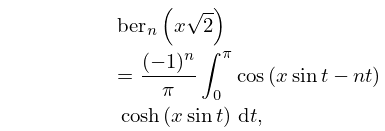
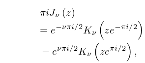
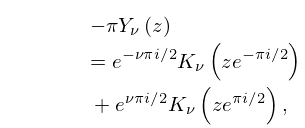
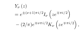
15: 10.64 Integral Representations

… ►

10.64.1 $${\mathrm{ber}}_n\left(x\sqrt{2}\right)=\frac{{(-1)}^n}{\pi }{\int }_0^{\pi }\cos \left(x\sin t-nt\right)\cosh \left(x\sin t\right)dt,$$

ⓘ

Symbols:

${\mathrm{ber}}_{\nu }\left(x\right)$: Kelvin function, $\pi$: the ratio of the circumference of a circle to its diameter, $\cos z$: cosine function, $dx$: differential of $x$ , $\cosh z$: hyperbolic cosine function, $\int$: integral, $\sin z$: sine function, $n$: integer and $x$: real variable

Permalink:

http://dlmf.nist.gov/10.64.E1

Encodings:

pMML, png, TeX

See also:

Annotations for §10.64, §10.64 and Ch.10

►

10.64.2 $${\mathrm{bei}}_n\left(x\sqrt{2}\right)=\frac{{(-1)}^n}{\pi }{\int }_0^{\pi }\sin \left(x\sin t-nt\right)\sinh \left(x\sin t\right)dt.$$

ⓘ

Symbols:

${\mathrm{bei}}_{\nu }\left(x\right)$: Kelvin function, $\pi$: the ratio of the circumference of a circle to its diameter, $dx$: differential of $x$ , $\sinh z$: hyperbolic sine function, $\int$: integral, $\sin z$: sine function, $n$: integer and $x$: real variable

Permalink:

http://dlmf.nist.gov/10.64.E2

Encodings:

pMML, png, TeX

See also:

Annotations for §10.64, §10.64 and Ch.10

…

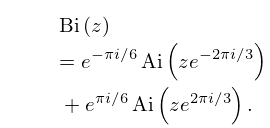
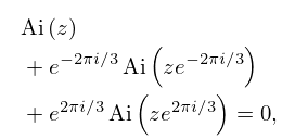
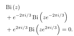
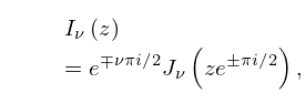
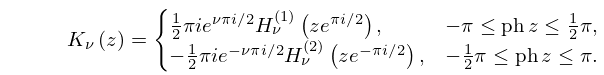
16: 10.61 Definitions and Basic Properties

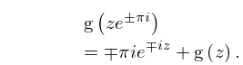
… ►In general, Kelvin functions have a branch point at $x=0$ and functions with arguments $x{\mathrm{e}}^{\pm \pi \mathrm{i}}$ are complex. … ►

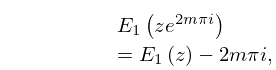
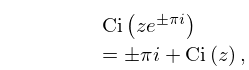
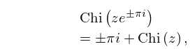
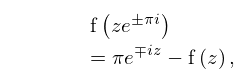
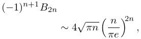
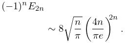
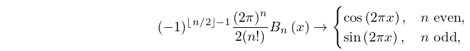
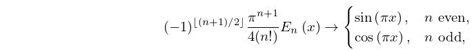
$${\mathrm{ber}}_{\frac{1}{2}}\left(x\sqrt{2}\right)=\frac{2^{-\frac{3}{4}}}{\sqrt{\pi x}}\left({\mathrm{e}}^x\cos \left(x+\frac{\pi }{8}\right)-{\mathrm{e}}^{-x}\cos \left(x-\frac{\pi }{8}\right)\right),$$

►

$${\mathrm{bei}}_{\frac{1}{2}}\left(x\sqrt{2}\right)=\frac{2^{-\frac{3}{4}}}{\sqrt{\pi x}}\left({\mathrm{e}}^x\sin \left(x+\frac{\pi }{8}\right)+{\mathrm{e}}^{-x}\sin \left(x-\frac{\pi }{8}\right)\right).$$

►

$${\mathrm{ber}}_{-\frac{1}{2}}\left(x\sqrt{2}\right)=\frac{2^{-\frac{3}{4}}}{\sqrt{\pi x}}\left({\mathrm{e}}^x\sin \left(x+\frac{\pi }{8}\right)-{\mathrm{e}}^{-x}\sin \left(x-\frac{\pi }{8}\right)\right),$$

►

$${\mathrm{bei}}_{-\frac{1}{2}}\left(x\sqrt{2}\right)=-\frac{2^{-\frac{3}{4}}}{\sqrt{\pi x}}\left({\mathrm{e}}^x\cos \left(x+\frac{\pi }{8}\right)+{\mathrm{e}}^{-x}\cos \left(x-\frac{\pi }{8}\right)\right).$$

…

17: 9.2 Differential Equation

… ►

9.2.10 $$\mathrm{Bi}\left(z\right)={\mathrm{e}}^{-\pi \mathrm{i}/6}\mathrm{Ai}\left(z{\mathrm{e}}^{-2\pi \mathrm{i}/3}\right)+{\mathrm{e}}^{\pi \mathrm{i}/6}\mathrm{Ai}\left(z{\mathrm{e}}^{2\pi \mathrm{i}/3}\right).$$

ⓘ

Symbols:

$\mathrm{Ai}\left(z\right)$: Airy function, $\mathrm{Bi}\left(z\right)$: Airy function, $\pi$: the ratio of the circumference of a circle to its diameter, $\mathrm{e}$: base of natural logarithm, $\mathrm{i}$: imaginary unit and $z$: complex variable

Proof sketch:

Derivable from Olver (1997b, p. 414).

A&S Ref:

10.4.6

Referenced by:

(9.10.19), (9.5.5)

Permalink:

http://dlmf.nist.gov/9.2.E10

Encodings:

pMML, png, TeX

See also:

Annotations for §9.2(v), §9.2 and Ch.9

… ►

9.2.12 $$\mathrm{Ai}\left(z\right)+{\mathrm{e}}^{-2\pi \mathrm{i}/3}\mathrm{Ai}\left(z{\mathrm{e}}^{-2\pi \mathrm{i}/3}\right)+{\mathrm{e}}^{2\pi \mathrm{i}/3}\mathrm{Ai}\left(z{\mathrm{e}}^{2\pi \mathrm{i}/3}\right)=0,$$

ⓘ

Symbols:

$\mathrm{Ai}\left(z\right)$: Airy function, $\pi$: the ratio of the circumference of a circle to its diameter, $\mathrm{e}$: base of natural logarithm, $\mathrm{i}$: imaginary unit and $z$: complex variable

Source:

Olver (1997b, (8.03), p. 414)

A&S Ref:

10.4.7

Permalink:

http://dlmf.nist.gov/9.2.E12

Encodings:

pMML, png, TeX

See also:

Annotations for §9.2(v), §9.2 and Ch.9

►

9.2.13 $$\mathrm{Bi}\left(z\right)+{\mathrm{e}}^{-2\pi \mathrm{i}/3}\mathrm{Bi}\left(z{\mathrm{e}}^{-2\pi \mathrm{i}/3}\right)+{\mathrm{e}}^{2\pi \mathrm{i}/3}\mathrm{Bi}\left(z{\mathrm{e}}^{2\pi \mathrm{i}/3}\right)=0.$$

ⓘ

Symbols:

$\mathrm{Bi}\left(z\right)$: Airy function, $\pi$: the ratio of the circumference of a circle to its diameter, $\mathrm{e}$: base of natural logarithm, $\mathrm{i}$: imaginary unit and $z$: complex variable

Proof sketch:

Derivable from Olver (1997b, p. 414).

A&S Ref:

10.4.8

Permalink:

http://dlmf.nist.gov/9.2.E13

Encodings:

pMML, png, TeX

See also:

Annotations for §9.2(v), §9.2 and Ch.9

►

9.2.14 $$\mathrm{Ai}\left(-z\right)={\mathrm{e}}^{\pi \mathrm{i}/3}\mathrm{Ai}\left(z{\mathrm{e}}^{\pi \mathrm{i}/3}\right)+{\mathrm{e}}^{-\pi \mathrm{i}/3}\mathrm{Ai}\left(z{\mathrm{e}}^{-\pi \mathrm{i}/3}\right),$$

ⓘ

Symbols:

$\mathrm{Ai}\left(z\right)$: Airy function, $\pi$: the ratio of the circumference of a circle to its diameter, $\mathrm{e}$: base of natural logarithm, $\mathrm{i}$: imaginary unit and $z$: complex variable

Source:

Olver (1997b, p. 414)

Permalink:

http://dlmf.nist.gov/9.2.E14

Encodings:

pMML, png, TeX

See also:

Annotations for §9.2(v), §9.2 and Ch.9

►

9.2.15 $$\mathrm{Bi}\left(-z\right)={\mathrm{e}}^{-\pi \mathrm{i}/6}\mathrm{Ai}\left(z{\mathrm{e}}^{\pi \mathrm{i}/3}\right)+{\mathrm{e}}^{\pi \mathrm{i}/6}\mathrm{Ai}\left(z{\mathrm{e}}^{-\pi \mathrm{i}/3}\right).$$

ⓘ

Symbols:

$\mathrm{Ai}\left(z\right)$: Airy function, $\mathrm{Bi}\left(z\right)$: Airy function, $\pi$: the ratio of the circumference of a circle to its diameter, $\mathrm{e}$: base of natural logarithm, $\mathrm{i}$: imaginary unit and $z$: complex variable

Source:

Olver (1997b, p. 414)

Permalink:

http://dlmf.nist.gov/9.2.E15

Encodings:

pMML, png, TeX

See also:

Annotations for §9.2(v), §9.2 and Ch.9

…

18: 10.27 Connection Formulas

… ►

10.27.6 $$I_{\nu }\left(z\right)={\mathrm{e}}^{\mp \nu \pi \mathrm{i}/2}{J}_{\nu }\left(z{\mathrm{e}}^{\pm \pi \mathrm{i}/2}\right),$$ $-\pi \le \pm \mathrm{ph}z\le \frac{1}{2}\pi$,

ⓘ

Symbols:

$J_{\nu }\left(z\right)$: Bessel function of the first kind, $\pi$: the ratio of the circumference of a circle to its diameter, $\mathrm{e}$: base of natural logarithm, $\mathrm{i}$: imaginary unit, $I_{\nu }\left(z\right)$: modified Bessel function of the first kind, $\mathrm{ph}$: phase, $z$: complex variable and $\nu$: complex parameter

A&S Ref:

9.6.3 (modified)

Referenced by:

§10.26(ii), §10.27, §10.27, §10.31, §10.33, §10.35, §10.39, §10.41(i), §10.42, §10.43(ii), §10.43(iv), §10.44(i), §10.44(ii), §10.44(iii), §10.47(iv), §10.67(i), §11.4(i)

Permalink:

http://dlmf.nist.gov/10.27.E6

Encodings:

pMML, png, TeX

See also:

Annotations for §10.27 and Ch.10

… ►

10.27.8

ⓘ

Symbols:

$H_{\nu }^{(1)}\left(z\right)$: Bessel function of the third kind (or Hankel function), $H_{\nu }^{(2)}\left(z\right)$: Bessel function of the third kind (or Hankel function), $\pi$: the ratio of the circumference of a circle to its diameter, $\mathrm{e}$: base of natural logarithm, $\mathrm{i}$: imaginary unit, $K_{\nu }\left(z\right)$: modified Bessel function of the second kind, $\mathrm{ph}$: phase, $z$: complex variable and $\nu$: complex parameter

A&S Ref:

9.6.4

Referenced by:

§10.16, §10.26(ii), §10.27, §10.27, §10.32(ii), §10.39, §10.40(ii), §10.40(iii), §10.41(i), §10.42, §10.43(ii), §10.44(i), §10.44(ii), §10.44(iii), §10.47(iv), (9.7.16), §9.7(iii)

Permalink:

http://dlmf.nist.gov/10.27.E8

Encodings:

pMML, png, TeX

See also:

Annotations for §10.27 and Ch.10

►

10.27.9 $$\pi \mathrm{i}{J}_{\nu }\left(z\right)={\mathrm{e}}^{-\nu \pi \mathrm{i}/2}{K}_{\nu }\left(z{\mathrm{e}}^{-\pi \mathrm{i}/2}\right)-{\mathrm{e}}^{\nu \pi \mathrm{i}/2}{K}_{\nu }\left(z{\mathrm{e}}^{\pi \mathrm{i}/2}\right),$$ $|\mathrm{ph}z|\le \frac{1}{2}\pi$.

ⓘ

Symbols:

$J_{\nu }\left(z\right)$: Bessel function of the first kind, $\pi$: the ratio of the circumference of a circle to its diameter, $\mathrm{e}$: base of natural logarithm, $\mathrm{i}$: imaginary unit, $K_{\nu }\left(z\right)$: modified Bessel function of the second kind, $\mathrm{ph}$: phase, $z$: complex variable and $\nu$: complex parameter

Referenced by:

§10.67(i)

Permalink:

http://dlmf.nist.gov/10.27.E9

Encodings:

pMML, png, TeX

See also:

Annotations for §10.27 and Ch.10

►

10.27.10 $$-\pi Y_{\nu }\left(z\right)={\mathrm{e}}^{-\nu \pi \mathrm{i}/2}{K}_{\nu }\left(z{\mathrm{e}}^{-\pi \mathrm{i}/2}\right)+{\mathrm{e}}^{\nu \pi \mathrm{i}/2}{K}_{\nu }\left(z{\mathrm{e}}^{\pi \mathrm{i}/2}\right),$$ $|\mathrm{ph}z|\le \frac{1}{2}\pi$.

ⓘ

Symbols:

$Y_{\nu }\left(z\right)$: Bessel function of the second kind, $\pi$: the ratio of the circumference of a circle to its diameter, $\mathrm{e}$: base of natural logarithm, $\mathrm{i}$: imaginary unit, $K_{\nu }\left(z\right)$: modified Bessel function of the second kind, $\mathrm{ph}$: phase, $z$: complex variable and $\nu$: complex parameter

Referenced by:

§10.43(iv)

Permalink:

http://dlmf.nist.gov/10.27.E10

Encodings:

pMML, png, TeX

See also:

Annotations for §10.27 and Ch.10

►

10.27.11 $$Y_{\nu }\left(z\right)={\mathrm{e}}^{\pm (\nu +1)\pi \mathrm{i}/2}{I}_{\nu }\left(z{\mathrm{e}}^{\mp \pi \mathrm{i}/2}\right)-(2/\pi ){\mathrm{e}}^{\mp \nu \pi \mathrm{i}/2}{K}_{\nu }\left(z{\mathrm{e}}^{\mp \pi \mathrm{i}/2}\right),$$ $-\frac{1}{2}\pi \le \pm \mathrm{ph}z\le \pi$.

ⓘ

Symbols:

$Y_{\nu }\left(z\right)$: Bessel function of the second kind, $\pi$: the ratio of the circumference of a circle to its diameter, $\mathrm{e}$: base of natural logarithm, $\mathrm{i}$: imaginary unit, $I_{\nu }\left(z\right)$: modified Bessel function of the first kind, $K_{\nu }\left(z\right)$: modified Bessel function of the second kind, $\mathrm{ph}$: phase, $z$: complex variable and $\nu$: complex parameter

A&S Ref:

9.6.5 (modified)

Referenced by:

§11.6(i)

Permalink:

http://dlmf.nist.gov/10.27.E11

Encodings:

pMML, png, TeX

See also:

Annotations for §10.27 and Ch.10

…

19: 24.9 Inequalities

… ►

24.9.6 $$5\sqrt{\pi n}{\left(\frac{n}{\pi \mathrm{e}}\right)}^{2n}>{(-1)}^{n+1}{B}_{2n}>4\sqrt{\pi n}{\left(\frac{n}{\pi \mathrm{e}}\right)}^{2n},$$

ⓘ

Symbols:

$B_n$: Bernoulli numbers, $\pi$: the ratio of the circumference of a circle to its diameter, $\mathrm{e}$: base of natural logarithm and $n$: integer

Referenced by:

§24.9, §24.9

Permalink:

http://dlmf.nist.gov/24.9.E6

Encodings:

pMML, png, TeX

See also:

Annotations for §24.9 and Ch.24

►

24.9.7 $$8\sqrt{\frac{n}{\pi }}{\left(\frac{4n}{\pi \mathrm{e}}\right)}^{2n}\left(1+\frac{1}{12n}\right)>{(-1)}^n{E}_{2n}>8\sqrt{\frac{n}{\pi }}{\left(\frac{4n}{\pi \mathrm{e}}\right)}^{2n}.$$

ⓘ

Symbols:

$E_n$: Euler numbers, $\pi$: the ratio of the circumference of a circle to its diameter, $\mathrm{e}$: base of natural logarithm and $n$: integer

Referenced by:

§24.9, §24.9

Permalink:

http://dlmf.nist.gov/24.9.E7

Encodings:

pMML, png, TeX

See also:

Annotations for §24.9 and Ch.24

… ►

24.9.8 $$\frac{2(2n)!}{{(2\pi )}^{2n}}\frac{1}{1-2^{\beta -2n}}\ge {(-1)}^{n+1}{B}_{2n}\ge \frac{2(2n)!}{{(2\pi )}^{2n}}\frac{1}{1-2^{-2n}}$$

ⓘ

Symbols:

$B_n$: Bernoulli numbers, $\pi$: the ratio of the circumference of a circle to its diameter, $!$: factorial (as in $n!$), $n$: integer and $\beta$: quantity

Referenced by:

§24.9

Permalink:

http://dlmf.nist.gov/24.9.E8

Encodings:

pMML, png, TeX

See also:

Annotations for §24.9 and Ch.24

… ►

24.9.9 $$\beta =2+\frac{\ln \left(1-6{\pi }^{-2}\right)}{\ln 2}=0.6491\mathrm{\dots }.$$

ⓘ

Symbols:

$\pi$: the ratio of the circumference of a circle to its diameter, $\ln z$: principal branch of logarithm function and $\beta$: quantity

Permalink:

http://dlmf.nist.gov/24.9.E9

Encodings:

pMML, png, TeX

See also:

Annotations for §24.9 and Ch.24

►

24.9.10 $$\frac{4^{n+1}(2n)!}{{\pi }^{2n+1}}>{(-1)}^n{E}_{2n}>\frac{4^{n+1}(2n)!}{{\pi }^{2n+1}}\frac{1}{1+3^{-1-2n}}.$$

ⓘ

Symbols:

$E_n$: Euler numbers, $\pi$: the ratio of the circumference of a circle to its diameter, $!$: factorial (as in $n!$) and $n$: integer

A&S Ref:

23.1.15

Referenced by:

§24.9

Permalink:

http://dlmf.nist.gov/24.9.E10

Encodings:

pMML, png, TeX

See also:

Annotations for §24.9 and Ch.24

20: 11.8 Analogs to Kelvin Functions

§11.8 Analogs to Kelvin Functions

►For properties of Struve functions of argument $x{\mathrm{e}}^{\pm 3\pi \mathrm{i}/4}$ see McLachlan and Meyers (1936).