Clausen integral

SearchAdvancedHelp

(0.001 seconds)

7 matching pages

1: 25.19 Tables

… ►

Abramowitz and Stegun (1964) tabulates: $\zeta \left(n\right)$, $n=2,3,4,\mathrm{\dots }$, 20D (p. 811); ${\mathrm{Li}}_2\left(1-x\right)$, $x=0(.01)0.5$, 9D (p. 1005); $f(\theta )$, $\theta ={15}^{\circ }(1^{\circ }){30}^{\circ }(2^{\circ }){90}^{\circ }(5^{\circ }){180}^{\circ }$, $f(\theta )+\theta \ln \theta$, $\theta =0(1^{\circ }){15}^{\circ }$, 6D (p. 1006). Here $f(\theta )$ denotes Clausen’s integral, given by the right-hand side of (25.12.9).

… ►

Cloutman (1989) tabulates $\mathrm{\Gamma }\left(s+1\right)F_s(x)$, where $F_s(x)$ is the Fermi–Dirac integral (25.12.14), for $s=-\frac{1}{2},\frac{1}{2},\frac{3}{2},\frac{5}{2}$, $x=-5(.05)25$, to 12S.

►

Fletcher et al. (1962, §22.1) lists many sources for earlier tables of $\zeta \left(s\right)$ for both real and complex $s$. §22.133 gives sources for numerical values of coefficients in the Riemann–Siegel formula, §22.15 describes tables of values of $\zeta (s,a)$, and §22.17 lists tables for some Dirichlet $L$-functions for real characters. For tables of dilogarithms, polylogarithms, and Clausen’s integral see §§22.84–22.858.

2: 25.21 Software

… ►

§25.21(vi) Clausen’s Integral

…

3: 25.12 Polylogarithms

… ►

25.12.9 $$\sum _{n=1}^{\mathrm{\infty }}\frac{\sin \left(n\theta \right)}{n^2}=-{\int }_0^{\theta }\ln \left(2\sin \left(\frac{1}{2}x\right)\right)dx.$$

ⓘ

Symbols:

$dx$: differential of $x$ , $\int$: integral, $\ln z$: principal branch of logarithm function, $\sin z$: sine function, $n$: nonnegative integer, $x$: real variable and $\theta$: phase

Keywords:

definite integral, infinite series

Source:

Maximon (2003, (8.7), (8.8), p. 2813)

A&S Ref:

27.8.6 (integration of first series)

Referenced by:

1st item

Permalink:

http://dlmf.nist.gov/25.12.E9

Encodings:

pMML, png, TeX

See also:

Annotations for §25.12(i), §25.12 and Ch.25

►The right-hand side is called Clausen’s integral. …

4: Software Index

… ► ►►►

	Open Source													With Book						Commercial
…
25.21(vi) Clausen’s Integral					✓				✓			a	✓									✓			NetNUMPAC
…

…

5: Bibliography K

… ►

On an integral of Hardy and Littlewood. Kyushu J. Math. 52 (1), pp. 249–263.

ⓘ

External Links:

ISSN 1340-6116, Document, MathReview (Fritz Haslinger), ZentralBlatt

Referenced by:

§9.13(ii).

Encodings:

BibTeX

… ►

Auxiliary table for the incomplete elliptic integrals. J. Math. Physics 27, pp. 11–36.

ⓘ

External Links:

MathReview (S. C. van Veen), ZentralBlatt

Referenced by:

§19.12.

Encodings:

BibTeX

… ►

The congruences of Clausen-von Staudt and Kummer for Bernoulli-Hurwitz numbers. Math. Ann. 216 (1), pp. 1–4.

ⓘ

External Links:

ISSN 0025-5831, Document, MathReview (M. Basmakov), ZentralBlatt

Referenced by:

§24.16(iii).

Encodings:

BibTeX

… ►

An indirect method for evaluating certain infinite integrals. Z. Angew. Math. Phys. 29 (3), pp. 380–386.

ⓘ

External Links:

ISSN 0044-2275, Document, MathReview, ZentralBlatt

Referenced by:

§10.71(ii).

Encodings:

BibTeX

… ►

On the zeros of the Fresnel integrals. Canad. J. Math. 9, pp. 118–131.

ⓘ

External Links:

MathReview (W. C. Rheinboldt), ZentralBlatt

Referenced by:

§7.13(iii).

Encodings:

BibTeX

…

6: Bibliography C

… ►

The Staudt-Clausen theorem. Math. Mag. 34, pp. 131–146.

ⓘ

External Links:

MathReview (K. Goldberg), ZentralBlatt

Referenced by:

§24.6.

Encodings:

BibTeX

… ►

On computing elliptic integrals and functions. J. Math. and Phys. 44, pp. 36–51.

ⓘ

External Links:

MathReview (R. Nicolovius), ZentralBlatt

Referenced by:

§19.36(ii), §19.36(ii).

Encodings:

BibTeX

… ►

Inequalities for a symmetric elliptic integral. Proc. Amer. Math. Soc. 25 (3), pp. 698–703.

ⓘ

External Links:

FullText, MathReview (Y. L. Luke), ZentralBlatt

Referenced by:

§19.24(ii), §19.9(ii).

Encodings:

BibTeX

… ►

Über die Fälle, wenn die Reihe von der Form $y=1+\frac{\alpha }{1}\cdot \frac{\beta }{\gamma }x+\frac{\alpha \cdot \alpha +1}{1\cdot 2}\cdot \frac{\beta \cdot \beta +1}{\gamma \cdot \gamma +1}{x}^2+$ etc. ein Quadrat von der Form $z=1+\frac{{\alpha }^{\prime }}{1}\cdot \frac{{\beta }^{\prime }}{{\gamma }^{\prime }}\cdot \frac{{\delta }^{\prime }}{{ϵ}^{\prime }}x+\frac{{\alpha }^{\prime }\cdot {\alpha }^{\prime }+1}{1\cdot 2}\cdot \frac{{\beta }^{\prime }\cdot {\beta }^{\prime }+1}{{\gamma }^{\prime }\cdot {\gamma }^{\prime }+1}\cdot \frac{{\delta }^{\prime }\cdot {\delta }^{\prime }+1}{{ϵ}^{\prime }\cdot {ϵ}^{\prime }+1}{x}^2+$ etc. hat. J. Reine Angew. Math. 3, pp. 89–91.

ⓘ

External Links:

Link, MathReview Entry, ZentralBlatt

Referenced by:

§16.12.

Encodings:

BibTeX

… ►

Integrals involving complete elliptic integrals. J. Comput. Appl. Math. 106 (1), pp. 169–175.

ⓘ

External Links:

ISSN 0377-0427, Document, MathReview, ZentralBlatt

Referenced by:

§19.13(i).

Encodings:

BibTeX

…

7: Errata

… ►

The title of the paragraph which was previously “Gasper’s $q$-Analog of Clausen’s Formula” has been changed to “Gasper’s $q$-Analog of Clausen’s Formula (16.12.2)”.

… ►

Scales were corrected in all figures. The interval $-8.4\le \frac{x-y}{\sqrt{2}}\le 8.4$ was replaced by $-12.0\le \frac{x-y}{\sqrt{2}}\le 12.0$ and $-12.7\le \frac{x+y}{\sqrt{2}}\le 4.2$ replaced by $-18.0\le \frac{x+y}{\sqrt{2}}\le 6.0$. All plots and interactive visualizations were regenerated to improve image quality.

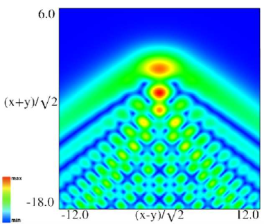
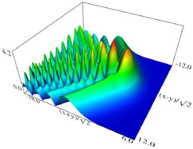
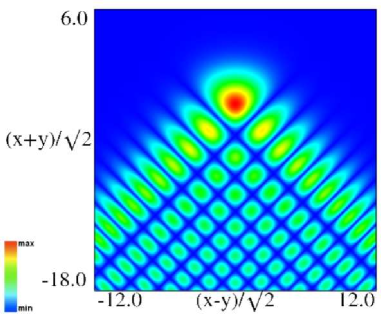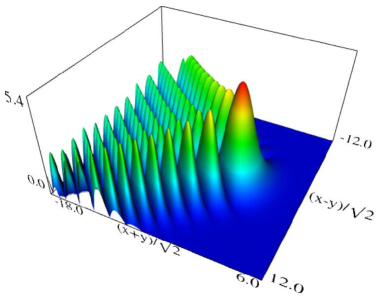(a) Density plot.	(b) 3D plot.

Figure 36.3.9: Modulus of hyperbolic umbilic canonical integral function $|{\mathrm{\Psi }}^{(\mathrm{H})}\left(x,y,0\right)|$.

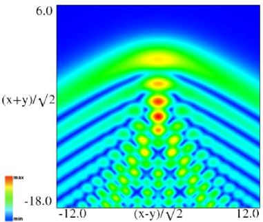
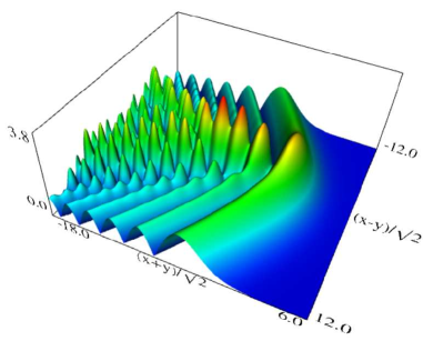
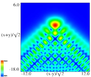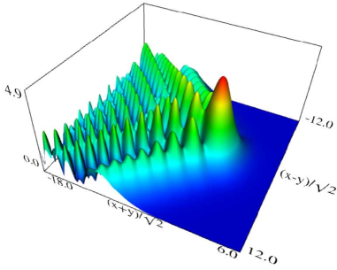(a) Density plot.	(b) 3D plot.

Figure 36.3.10: Modulus of hyperbolic umbilic canonical integral function $|{\mathrm{\Psi }}^{(\mathrm{H})}\left(x,y,1\right)|$.

(a) Density plot.	(b) 3D plot.

Figure 36.3.11: Modulus of hyperbolic umbilic canonical integral function $|{\mathrm{\Psi }}^{(\mathrm{H})}\left(x,y,2\right)|$.

(a) Density plot.	(b) 3D plot.

Figure 36.3.12: Modulus of hyperbolic umbilic canonical integral function $|{\mathrm{\Psi }}^{(\mathrm{H})}\left(x,y,3\right)|$.

Reported 2016-09-12 by Dan Piponi.

►

The scaling error reported on 2016-09-12 by Dan Piponi also applied to contour and density plots for the phase of the hyperbolic umbilic canonical integrals. Scales were corrected in all figures. The interval $-8.4\le \frac{x-y}{\sqrt{2}}\le 8.4$ was replaced by $-12.0\le \frac{x-y}{\sqrt{2}}\le 12.0$ and $-12.7\le \frac{x+y}{\sqrt{2}}\le 4.2$ replaced by $-18.0\le \frac{x+y}{\sqrt{2}}\le 6.0$. All plots and interactive visualizations were regenerated to improve image quality.

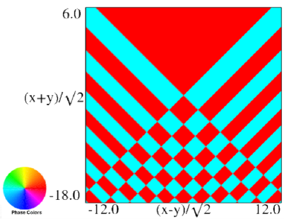(a) Contour plot.	(b) Density plot.

Figure 36.3.18: Phase of hyperbolic umbilic canonical integral $\mathrm{ph}{\mathrm{\Psi }}^{(\mathrm{H})}\left(x,y,0\right)$.

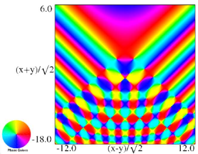(a) Contour plot.	(b) Density plot.

Figure 36.3.19: Phase of hyperbolic umbilic canonical integral $\mathrm{ph}{\mathrm{\Psi }}^{(\mathrm{H})}\left(x,y,1\right)$.

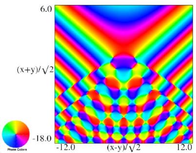(a) Contour plot.	(b) Density plot.

Figure 36.3.20: Phase of hyperbolic umbilic canonical integral $\mathrm{ph}{\mathrm{\Psi }}^{(\mathrm{H})}\left(x,y,2\right)$.

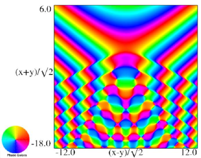(a) Contour plot.	(b) Density plot.

Figure 36.3.21: Phase of hyperbolic umbilic canonical integral $\mathrm{ph}{\mathrm{\Psi }}^{(\mathrm{H})}\left(x,y,3\right)$.

Reported 2016-09-28.

… ►

36.10.14 $$3\left(\frac{{\partial }^2{\mathrm{\Psi }}^{(\mathrm{E})}}{{\partial x}^2}-\frac{{\partial }^2{\mathrm{\Psi }}^{(\mathrm{E})}}{{\partial y}^2}\right)+2\mathrm{i}z\frac{\partial {\mathrm{\Psi }}^{(\mathrm{E})}}{\partial x}-x{\mathrm{\Psi }}^{(\mathrm{E})}=0$$

Originally this equation appeared with $\frac{\partial {\mathrm{\Psi }}^{(\mathrm{H})}}{\partial x}$ in the second term, rather than $\frac{\partial {\mathrm{\Psi }}^{(\mathrm{E})}}{\partial x}$.

Reported 2010-04-02.

… ►

The definition of $R_C(x,y)$ was revised in Notations.

…