Bailey 2F1(-1) sum

SearchAdvancedHelp

(0.014 seconds)

21—30 of 817 matching pages

21: 22.18 Mathematical Applications

… ►In polar coordinates, $x=r\cos \varphi$, $y=r\sin \varphi$, the lemniscate is given by $r^2=\cos \left(2\varphi \right)$, $0\le \varphi \le 2\pi$. … ►With $k\in [0,1]$ the mapping $z\to w=\mathrm{sn}(z,k)$ gives a conformal map of the closed rectangle $[-K,K]\times [0,K^{\prime }]$ onto the half-plane $\mathrm{\Im }w\ge 0$, with $0,\pm K,\pm K+\mathrm{i}{K}^{\prime },\mathrm{i}{K}^{\prime }$ mapping to $0,\pm 1,\pm k^{-2},\mathrm{\infty }$ respectively. …See Akhiezer (1990, Chapter 8) and McKean and Moll (1999, Chapter 2) for discussions of the inverse mapping. … ►The special case $y^2=(1-x^2)(1-k^2{x}^2)$ is in Jacobian normal form. For any two points $(x_1,y_1)$ and $(x_2,y_2)$ on this curve, their sum $(x_3,y_3)$, always a third point on the curve, is defined by the Jacobi–Abel addition law …

22: 10.59 Integrals

… ►

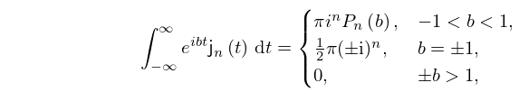
10.59.1

ⓘ

Symbols:

$P_n\left(x\right)$: Legendre polynomial, $\pi$: the ratio of the circumference of a circle to its diameter, $dx$: differential of $x$ , $\mathrm{e}$: base of natural logarithm, $\mathrm{i}$: imaginary unit, $\int$: integral, ${𝗃}_n\left(z\right)$: spherical Bessel function of the first kind and $n$: integer

A&S Ref:

11.4.26

Referenced by:

§10.59

Permalink:

http://dlmf.nist.gov/10.59.E1

Encodings:

pMML, png, TeX

See also:

Annotations for §10.59 and Ch.10

…

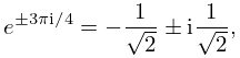
23: 4.4 Special Values and Limits

… ►

4.4.2 $$\ln \left(-1\pm \mathrm{i}0\right)=\pm \pi \mathrm{i},$$

ⓘ

Symbols:

$\pi$: the ratio of the circumference of a circle to its diameter, $\mathrm{i}$: imaginary unit and $\ln z$: principal branch of logarithm function

A&S Ref:

4.1.14 (modified)

Permalink:

http://dlmf.nist.gov/4.4.E2

Encodings:

pMML, png, TeX

See also:

Annotations for §4.4(i), §4.4 and Ch.4

►

4.4.3 $$\ln \left(\pm \mathrm{i}\right)=\pm \frac{1}{2}\pi \mathrm{i}.$$

ⓘ

Symbols:

$\pi$: the ratio of the circumference of a circle to its diameter, $\mathrm{i}$: imaginary unit and $\ln z$: principal branch of logarithm function

A&S Ref:

4.1.15

Permalink:

http://dlmf.nist.gov/4.4.E3

Encodings:

pMML, png, TeX

See also:

Annotations for §4.4(i), §4.4 and Ch.4

… ►

4.4.10 $${\mathrm{e}}^{\pm \pi \mathrm{i}/4}=\frac{1}{\sqrt{2}}\pm \mathrm{i}\frac{1}{\sqrt{2}},$$

ⓘ

Symbols:

$\pi$: the ratio of the circumference of a circle to its diameter, $\mathrm{e}$: base of natural logarithm and $\mathrm{i}$: imaginary unit

Permalink:

http://dlmf.nist.gov/4.4.E10

Encodings:

pMML, png, TeX

See also:

Annotations for §4.4(ii), §4.4 and Ch.4

►

4.4.11 $${\mathrm{e}}^{\pm 3\pi \mathrm{i}/4}=-\frac{1}{\sqrt{2}}\pm \mathrm{i}\frac{1}{\sqrt{2}},$$

ⓘ

Symbols:

$\pi$: the ratio of the circumference of a circle to its diameter, $\mathrm{e}$: base of natural logarithm and $\mathrm{i}$: imaginary unit

Permalink:

http://dlmf.nist.gov/4.4.E11

Encodings:

pMML, png, TeX

See also:

Annotations for §4.4(ii), §4.4 and Ch.4

… ►where $a$ ($\in ℂ$) and $\delta$ ($\in (0,\frac{1}{2}\pi ]$) are constants. …

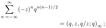
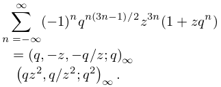
24: 17.8 Special Cases of ${}_r{}^{}\psi _r^{}$ Functions

… ►

17.8.1 $$\sum _{n=-\mathrm{\infty }}^{\mathrm{\infty }}{(-z)}^n{q}^{n(n-1)/2}={(q,z,q/z;q)}_{\mathrm{\infty }};$$

ⓘ

Symbols:

${(a_1,a_2,\mathrm{\dots },a_r;q)}_n$: multiple $q$-Pochhammer symbol, $q$: complex base, $n$: nonnegative integer and $z$: complex variable

Permalink:

http://dlmf.nist.gov/17.8.E1

Encodings:

pMML, png, TeX

See also:

Annotations for §17.8, §17.8 and Ch.17

… ►

17.8.3 $$\sum _{n=-\mathrm{\infty }}^{\mathrm{\infty }}{(-1)}^n{q}^{n(3n-1)/2}{z}^{3n}(1+z{q}^n)={(q,-z,-q/z;q)}_{\mathrm{\infty }}{(q{z}^2,q/z^2;q^2)}_{\mathrm{\infty }}.$$

ⓘ

Symbols:

${(a_1,a_2,\mathrm{\dots },a_r;q)}_n$: multiple $q$-Pochhammer symbol, $q$: complex base, $n$: nonnegative integer and $z$: complex variable

Permalink:

http://dlmf.nist.gov/17.8.E3

Encodings:

pMML, png, TeX

See also:

Annotations for §17.8, §17.8 and Ch.17

►

Bailey’s Bilateral Summations

… ►

Sum Related to (17.6.4)

►

17.8.8 $${}_2{}^{}\psi _2^{}(\genfrac{}{}{0pt}{}{b^2,b^2/c}{q,cq};q^2,c{q}^2/b^2)=\frac{1}{2}\frac{{(q^2,q{b}^2,q/b^2,cq/b^2;q^2)}_{\mathrm{\infty }}}{{(cq,c{q}^2/b^2,q^2/b^2,c/b^2;q^2)}_{\mathrm{\infty }}}\left(\frac{{(c\sqrt{q}/b;q)}_{\mathrm{\infty }}}{{(b\sqrt{q};q)}_{\mathrm{\infty }}}+\frac{{(-c\sqrt{q}/b;q)}_{\mathrm{\infty }}}{{(-b\sqrt{q};q)}_{\mathrm{\infty }}}\right),$$ .

ⓘ

Symbols:

${(a;q)}_n$: $q$-Pochhammer symbol (or $q$-shifted factorial), ${}_r{}^{}\psi _s^{}(a_1,\mathrm{\dots },a_r;b_1,\mathrm{\dots },b_s;q,z)$ or ${}_r{}^{}\psi _s^{}(\genfrac{}{}{0pt}{}{a_1,\mathrm{\dots },a_r}{b_1,\mathrm{\dots },b_s};q,z)$: bilateral basic hypergeometric (or bilateral $q$-hypergeometric) function, ${(a_1,a_2,\mathrm{\dots },a_r;q)}_n$: multiple $q$-Pochhammer symbol and $q$: complex base

Source:

Verma and Jain (1983, (3.9))

Referenced by:

§17.6(i), §17.8, Erratum (V1.1.0) for Additions

Permalink:

http://dlmf.nist.gov/17.8.E8

Encodings:

pMML, png, TeX

Addition (effective with 1.1.0):

This equation was added.

Suggested 2019-10-19 by Slobodan Damjanovic

See also:

Annotations for §17.8, §17.8 and Ch.17

…

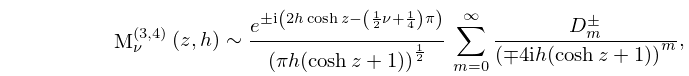
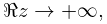
25: 28.25 Asymptotic Expansions for Large $\mathrm{\Re }z$

… ►

28.25.1 $${\mathrm{M}}_{\nu }^{(3,4)}(z,h)\sim \frac{{\mathrm{e}}^{\pm \mathrm{i}\left(2h\cosh z-\left(\frac{1}{2}\nu +\frac{1}{4}\right)\pi \right)}}{{\left(\pi h(\cosh z+1)\right)}^{\frac{1}{2}}}\sum _{m=0}^{\mathrm{\infty }}\frac{D_m^{\pm }}{{\left(\mp 4\mathrm{i}h(\cosh z+1)\right)}^m},$$

ⓘ

Symbols:

$\sim$: Poincaré asymptotic expansion, $\pi$: the ratio of the circumference of a circle to its diameter, $\mathrm{e}$: base of natural logarithm, $\cosh z$: hyperbolic cosine function, $\mathrm{i}$: imaginary unit, ${\mathrm{M}}_{\nu }^{(j)}(z,h)$: modified Mathieu function, $m$: integer, $h$: parameter, $z$: complex variable, $\nu$: complex parameter and $D_m^{\pm }$: coefficients

A&S Ref:

20.9.1 (for 3 and for integer $\nu$) 20.9.3 (for 4 and for integer $\nu$)

Referenced by:

§28.25

Permalink:

http://dlmf.nist.gov/28.25.E1

Encodings:

pMML, png, TeX

See also:

Annotations for §28.25 and Ch.28

… ►

$D_{-1}^{\pm }=0,$

►

$D_0^{\pm }=1,$

… ►

28.25.3 $$(m+1)D_{m+1}^{\pm }+\left({(m+\frac{1}{2})}^2\pm (m+\frac{1}{4})8\mathrm{i}h+2h^2-a\right)D_m^{\pm }\pm (m-\frac{1}{2})\left(8\mathrm{i}hm\right)D_{m-1}^{\pm }=0,$$ $m\ge 0$.

ⓘ

Symbols:

$\mathrm{i}$: imaginary unit, $m$: integer, $h$: parameter, $a$: parameter and $D_m^{\pm }$: coefficients

A&S Ref:

20.9.2 (for $+$) 20.9.4 (for $-$)

Permalink:

http://dlmf.nist.gov/28.25.E3

Encodings:

pMML, png, TeX

See also:

Annotations for §28.25 and Ch.28

… ►

28.25.4 $$\mathrm{\Re }z\to +\mathrm{\infty },$$ $-\pi +\delta \le \mathrm{ph}h+\mathrm{\Im }z\le 2\pi -\delta$,

ⓘ

Symbols:

$\pi$: the ratio of the circumference of a circle to its diameter, $\mathrm{\Im }$: imaginary part, $\mathrm{ph}$: phase, $\mathrm{\Re }$: real part, $h$: parameter, $z$: complex variable and $\delta$: arbitrary small positive constant

Permalink:

http://dlmf.nist.gov/28.25.E4

Encodings:

pMML, png, TeX

See also:

Annotations for §28.25 and Ch.28

…

26: 32.7 Bäcklund Transformations

… ►with $\zeta =-2^{1/3}z$ and $\epsilon =\pm 1$, where $W(\zeta ;\frac{1}{2}\epsilon )$ satisfies ${\text{P}}_{\text{II}}$ with $z=\zeta$, $\alpha =\frac{1}{2}\epsilon$, and $w(z;0)$ satisfies ${\text{P}}_{\text{II}}$ with $\alpha =0$. ►The solutions $w_{\alpha }=w(z;\alpha )$, $w_{\alpha \pm 1}=w(z;\alpha \pm 1)$, satisfy the nonlinear recurrence relation … ►and ${\epsilon }_j=\pm 1$, $j=1,2,3$, independently. …Again, since ${\epsilon }_j=\pm 1$, $j=1,2,3$, independently, there are eight distinct transformations of type ${𝒯}_{{\epsilon }_1,{\epsilon }_2,{\epsilon }_3}$. … ►with $\epsilon =\pm 1$. …

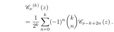
27: 10.6 Recurrence Relations and Derivatives

… ►

$H_0^{(1)}{}_{}{}^{\prime }\left(z\right)=-H_1^{(1)}\left(z\right),$ $H_0^{(2)}{}_{}{}^{\prime }\left(z\right)=-H_1^{(2)}\left(z\right).$

… ►For results on modified quotients of the form $z{𝒞}_{\nu \pm 1}\left(z\right)/{𝒞}_{\nu }\left(z\right)$ see Onoe (1955) and Onoe (1956). … ►For $k=0,1,2,\mathrm{\dots }$, … ►

10.6.7 $${𝒞}_{\nu }^{(k)}\left(z\right)=\frac{1}{2^k}\sum _{n=0}^k{(-1)}^n\left(\genfrac{}{}{0.0pt}{}{k}{n}\right){𝒞}_{\nu -k+2n}\left(z\right).$$

ⓘ

Symbols:

$\left(\genfrac{}{}{0.0pt}{}{m}{n}\right)$: binomial coefficient, ${𝒞}_{\nu }\left(z\right)$: cylinder function, $n$: integer, $k$: nonnegative integer, $z$: complex variable and $\nu$: complex parameter

A&S Ref:

9.1.31

Referenced by:

§10.6(ii)

Permalink:

http://dlmf.nist.gov/10.6.E7

Encodings:

pMML, png, TeX

See also:

Annotations for §10.6(ii), §10.6 and Ch.10

… ►

$s_{\nu }=\frac{1}{2}{p}_{\nu +1}+\frac{1}{2}{p}_{\nu -1}-{\displaystyle \frac{{\nu }^2}{ab}}{p}_{\nu },$

…

28: 17.1 Special Notation

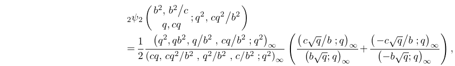
… ►The main functions treated in this chapter are the basic hypergeometric (or $q$-hypergeometric) function ${}_r{}^{}\varphi _s^{}(a_1,a_2,\mathrm{\dots },a_r;b_1,b_2,\mathrm{\dots },b_s;q,z)$, the bilateral basic hypergeometric (or bilateral $q$-hypergeometric) function ${}_r{}^{}\psi _s^{}(a_1,a_2,\mathrm{\dots },a_r;b_1,b_2,\mathrm{\dots },b_s;q,z)$, and the $q$-analogs of the Appell functions ${\mathrm{\Phi }}^{(1)}(a;b,b^{\prime };c;q;x,y)$, ${\mathrm{\Phi }}^{(2)}(a;b,b^{\prime };c,c^{\prime };q;x,y)$, ${\mathrm{\Phi }}^{(3)}(a,a^{\prime };b,b^{\prime };c;q;x,y)$, and ${\mathrm{\Phi }}^{(4)}(a,b;c,c^{\prime };q;x,y)$. … ►Another function notation used is the “idem” function: ►

$$f({\chi }_1;{\chi }_2,\mathrm{\dots },{\chi }_n)+\mathrm{idem}({\chi }_1;{\chi }_2,\mathrm{\dots },{\chi }_n)=\sum _{j=1}^{n}f({\chi }_j;{\chi }_1,{\chi }_2,\mathrm{\dots },{\chi }_{j-1},{\chi }_{j+1},\mathrm{\dots },{\chi }_n).$$

… ►A slightly different notation is that in Bailey (1964) and Slater (1966); see §17.4(i). Fine (1988) uses $F(a,b;t:q)$ for a particular specialization of a ${}_2{}^{}\varphi _1^{}$ function.

29: 15.4 Special Cases

… ►Exceptions are (15.4.8) and (15.4.10), that hold for , and (15.4.12), (15.4.14), and (15.4.16), that hold for . … ►

§15.4(ii) Argument Unity

… ►

Dougall’s Bilateral Sum

… ►

§15.4(iii) Other Arguments

… ►where the limit interpretation (15.2.6), rather than (15.2.5), has to be taken when in (15.4.33) $a=-\frac{1}{3},-\frac{4}{3},-\frac{7}{3},\mathrm{\dots }$, and in (15.4.34) $a=0,-1,-2,\mathrm{\dots }$. …

30: 4.37 Inverse Hyperbolic Functions

… ►In (4.37.1) the integration path may not pass through either of the points $t=\pm \mathrm{i}$, and the function ${(1+t^2)}^{1/2}$ assumes its principal value when $t$ is real. In (4.37.2) the integration path may not pass through either of the points $\pm 1$, and the function ${(t^2-1)}^{1/2}$ assumes its principal value when $t\in (1,\mathrm{\infty })$. …In (4.37.3) the integration path may not intersect $\pm 1$. …$\mathrm{Arcsinh}z$ and $\mathrm{Arccsch}z$ have branch points at $z=\pm \mathrm{i}$; the other four functions have branch points at $z=\pm 1$. … ►For example, $\mathrm{arcsech}a=\mathrm{arccoth}\left({(1-a^2)}^{-1/2}\right)$.