.世界杯各队主教练年薪『网址:mxsty.cc』.世界杯季军怎么算-m6q3s2-2022年12月1日13时59分20秒

SearchAdvancedHelp

(0.004 seconds)

11—20 of 837 matching pages

11: 3.4 Differentiation

… ►The Lagrange $(n+1)$-point formula is … ►where ${\xi }_0$ and ${\xi }_1\in I$. ►For the values of $n_0$ and $n_1$ used in the formulas below … ►

$$B_1^5=\frac{1}{12}(12+16t-21t^2-8t^3+5t^4),$$

… ►With the choice $r=k$ (which is crucial when $k$ is large because of numerical cancellation) the integrand equals ${\mathrm{e}}^k$ at the dominant points $\theta =0,2\pi$, and in combination with the factor $k^{-k}$ in front of the integral sign this gives a rough approximation to $1/k!$. …

12: 14.26 Uniform Asymptotic Expansions

… ►The uniform asymptotic approximations given in §14.15 for $P_{\nu }^{-\mu }\left(x\right)$ and ${𝑸}_{\nu }^{\mu }\left(x\right)$ for are extended to domains in the complex plane in the following references: §§14.15(i) and 14.15(ii), Dunster (2003b); §14.15(iii), Olver (1997b, Chapter 12); §14.15(iv), Boyd and Dunster (1986). …

13: 25.20 Approximations

… ►

Cody et al. (1971) gives rational approximations for $\zeta \left(s\right)$ in the form of quotients of polynomials or quotients of Chebyshev series. The ranges covered are $0.5\le s\le 5$, $5\le s\le 11$, $11\le s\le 25$, $25\le s\le 55$. Precision is varied, with a maximum of 20S.

►

Piessens and Branders (1972) gives the coefficients of the Chebyshev-series expansions of $s\zeta \left(s+1\right)$ and $\zeta \left(s+k\right)$, $k=2,3,4,5,8$, for $0\le s\le 1$ (23D).

►

Luke (1969b, p. 306) gives coefficients in Chebyshev-series expansions that cover $\zeta \left(s\right)$ for $0\le s\le 1$ (15D), $\zeta \left(s+1\right)$ for $0\le s\le 1$ (20D), and $\ln \xi \left(\frac{1}{2}+\mathrm{i}x\right)$ (§25.4) for $-1\le x\le 1$ (20D). For errata see Piessens and Branders (1972).

►

Morris (1979) gives rational approximations for ${\mathrm{Li}}_2\left(x\right)$ (§25.12(i)) for $0.5\le x\le 1$. Precision is varied with a maximum of 24S.

►

Antia (1993) gives minimax rational approximations for $\mathrm{\Gamma }\left(s+1\right)F_s(x)$, where $F_s(x)$ is the Fermi–Dirac integral (25.12.14), for the intervals and , with $s=-\frac{1}{2},\frac{1}{2},\frac{3}{2},\frac{5}{2}$. For each $s$ there are three sets of approximations, with relative maximum errors ${10}^{-4},{10}^{-8},{10}^{-12}$.

14: 34.11 Higher-Order $3nj$ Symbols

… ►For information on $12j,15j$,…, symbols, see Varshalovich et al. (1988, §10.12) and Yutsis et al. (1962, pp. 62–65 and 122–153).

15: 25.3 Graphics

… ►

►►

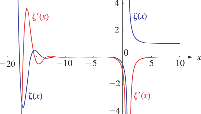
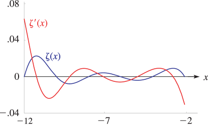
Figure 25.3.1: Riemann zeta function $\zeta \left(x\right)$ and its derivative ${\zeta }^{\prime }\left(x\right)$, $-20\le x\le 10$. Magnify

►

►►

Figure 25.3.2: Riemann zeta function $\zeta \left(x\right)$ and its derivative ${\zeta }^{\prime }\left(x\right)$, $-12\le x\le -2$. Magnify

… ►

►►

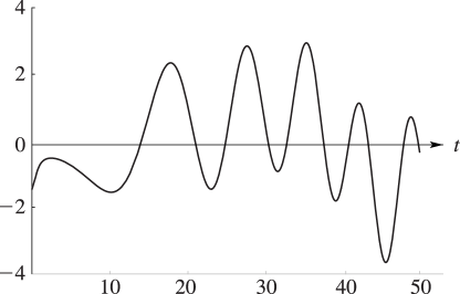
Figure 25.3.4: $Z(t)$, $0\le t\le 50$. $Z(t)$ and $\zeta \left(\frac{1}{2}+\mathrm{i}t\right)$ have the same zeros. … Magnify

…

16: 23.17 Elementary Properties

… ►

$J\left(\mathrm{i}\right)=1,$

… ►When … ►

23.17.6 $$\eta \left(\tau \right)=\sum _{n=-\mathrm{\infty }}^{\mathrm{\infty }}{(-1)}^n{q}^{{(6n+1)}^2/12}.$$

ⓘ

Symbols:

$\eta \left(\tau \right)$: Dedekind’s eta function (or Dedekind modular function), $q$: nome, $n$: integer and $\tau$: complex variable

Permalink:

http://dlmf.nist.gov/23.17.E6

Encodings:

pMML, png, TeX

See also:

Annotations for §23.17(ii), §23.17 and Ch.23

… ►

23.17.8 $$\eta \left(\tau \right)=q^{1/12}\prod _{n=1}^{\mathrm{\infty }}(1-q^{2n}),$$

ⓘ

Symbols:

$\eta \left(\tau \right)$: Dedekind’s eta function (or Dedekind modular function), $q$: nome, $n$: integer and $\tau$: complex variable

Referenced by:

§23.15(ii), §23.19

Permalink:

http://dlmf.nist.gov/23.17.E8

Encodings:

pMML, png, TeX

See also:

Annotations for §23.17(iii), §23.17 and Ch.23

►with $q^{1/12}={\mathrm{e}}^{\mathrm{i}\pi \tau /12}$.

17: 26.10 Integer Partitions: Other Restrictions

… ►Throughout this subsection it is assumed that . … ►where the sum is over nonnegative integer values of $k$ for which $n-\frac{1}{2}(3k^2\pm k)\ge 0$. … ►where the sum is over nonnegative integer values of $m$ for which $n-\frac{1}{2}k{m}^2-m+\frac{1}{2}km\ge 0$. … ►It is known that for $k>3$, $p(𝒟k,n)\ge p(\in A_{1,k+3},n)$, with strict inequality for $n$ sufficiently large, provided that $k=2^m-1,m=3,4,5$, or $k\ge 32$; see Yee (2004). … ►where $I_1\left(x\right)$ is the modified Bessel function (§10.25(ii)), and …

18: 26.2 Basic Definitions

… ►Thus $231$ is the permutation $\sigma (1)=2$, $\sigma (2)=3$, $\sigma (3)=1$. … ►As an example, $\{1,1,1,2,4,4\}$ is a partition of 13. …See Table 26.2.1 for $n=0(1)50$. For the actual partitions ($\pi$) for $n=1(1)5$ see Table 26.4.1. … ►The example $\{1,1,1,2,4,4\}$ has six parts, three of which equal 1. …

19: 26.21 Tables

… ►Andrews (1976) contains tables of the number of unrestricted partitions, partitions into odd parts, partitions into parts $\cancel{\equiv }\pm 2(mod5)$, partitions into parts $\cancel{\equiv }\pm 1(mod5)$, and unrestricted plane partitions up to 100. It also contains a table of Gaussian polynomials up to ${\left[\genfrac{}{}{0.0pt}{}{12}{6}\right]}_q$. …

20: 11.14 Tables

… ►

Abramowitz and Stegun (1964, Chapter 12) tabulates ${𝐇}_n\left(x\right)$, ${𝐇}_n\left(x\right)-Y_n\left(x\right)$, and $I_n\left(x\right)-{𝐋}_n\left(x\right)$ for $n=0,1$ and $x=0(.1)5$, $x^{-1}=0(.01)0.2$ to 6D or 7D.

… ►

Zanovello (1975) tabulates ${𝐇}_n\left(x\right)$ for $n=-4(1)15$ and $x=0.5(.5)26$ to 8D or 9S.

►

Zhang and Jin (1996) tabulates ${𝐇}_n\left(x\right)$ and ${𝐋}_n\left(x\right)$ for $n=-4(1)3$ and $x=0(1)20$ to 8D or 7S.

… ►

Abramowitz and Stegun (1964, Chapter 12) tabulates ${\int }_0^x(I_0\left(t\right)-{𝐋}_0\left(t\right))dt$ and $(2/\pi ){\int }_x^{\mathrm{\infty }}{t}^{-1}{𝐇}_0\left(t\right)dt$ for $x=0(.1)5$ to 5D or 7D; ${\int }_0^x({𝐇}_0\left(t\right)-Y_0\left(t\right))dt-(2/\pi )\ln x$, ${\int }_0^x(I_0\left(t\right)-{𝐋}_0\left(t\right))dt-(2/\pi )\ln x$, and ${\int }_x^{\mathrm{\infty }}{t}^{-1}({𝐇}_0\left(t\right)-Y_0\left(t\right))dt$ for $x^{-1}=0(.01)0.2$ to 6D.

… ►

Jahnke and Emde (1945) tabulates ${𝐄}_n\left(x\right)$ for $n=1,2$ and $x=0(.01)14.99$ to 4D.

…