www.rxlara.net - Stromectol tablets 3,6,12mg for SALE. Can I Buy Ivermectin without prescription. enter RXLARA.NET

SearchAdvancedHelp

(0.005 seconds)

21—30 of 743 matching pages

21: 8.26 Tables

… ►

Pearson (1965) tabulates the function $I(u,p)$ ($=P(p+1,u)$) for $p=-1(.05)0(.1)5(.2)50$, $u=0(.1)u_p$ to 7D, where $I(u,u_p)$ rounds off to 1 to 7D; also $I(u,p)$ for $p=-0.75(.01)-1$, $u=0(.1)6$ to 5D.

►

Zhang and Jin (1996, Table 3.8) tabulates $\gamma (a,x)$ for $a=0.5,1,3,5,10,25,50,100$, $x=0(.1)1(1)3,5(5)30,50,100$ to 8D or 8S.

… ►

Zhang and Jin (1996, Table 3.9) tabulates $I_x(a,b)$ for $x=0(.05)1$, $a=0.5,1,3,5,10$, $b=1,10$ to 8D.

… ►

Pagurova (1961) tabulates $E_n\left(x\right)$ for $n=0(1)20$, $x=0(.01)2(.1)10$ to 4-9S; ${\mathrm{e}}^x{E}_n\left(x\right)$ for $n=2(1)10$, $x=10(.1)20$ to 7D; ${\mathrm{e}}^x{E}_p\left(x\right)$ for $p=0(.1)1$, $x=0.01(.01)7(.05)12(.1)20$ to 7S or 7D.

… ►

Zhang and Jin (1996, Table 19.1) tabulates $E_n\left(x\right)$ for $n=1,2,3,5,10,15,20$, $x=0(.1)1,1.5,2,3,5,10,20,30,50,100$ to 7D or 8S.

22: 34.14 Tables

§34.14 Tables

►Tables of exact values of the squares of the $\mathit{3}j$ and $\mathit{6}j$ symbols in which all parameters are $\le 8$ are given in Rotenberg et al. (1959), together with a bibliography of earlier tables of $\mathit{3}j,\mathit{6}j$, and $\mathit{9}j$ symbols on pp. … ►Tables of $\mathit{3}j$ and $\mathit{6}j$ symbols in which all parameters are $\le 17/2$ are given in Appel (1968) to 6D. … 11-12; for $\mathit{6}j$ symbols on pp. … ► 270–289; similar tables for the $\mathit{6}j$ symbols are given on pp. …

23: 26.13 Permutations: Cycle Notation

… ►is $\left(1,3,2,5,7\right)\left(4\right)\left(6,8\right)$ in cycle notation. …In consequence, (26.13.2) can also be written as $\left(1,3,2,5,7\right)\left(6,8\right)$. … ►A permutation with cycle type $\left(a_1,a_2,\mathrm{\dots },a_n\right)$ can be written as a product of $a_2+2a_3+\mathrm{\cdots }+(n-1)a_n=n-(a_1+a_2+\mathrm{\cdots }+a_n)$ transpositions, and no fewer. For the example (26.13.2), this decomposition is given by $\left(1,3,2,5,7\right)\left(6,8\right)=\left(1,3\right)\left(2,3\right)\left(2,5\right)\left(5,7\right)\left(6,8\right).$ … ►Again, for the example (26.13.2) a minimal decomposition into adjacent transpositions is given by $\left(1,3,2,5,7\right)\left(6,8\right)=\left(2,3\right)\left(1,2\right)\left(4,5\right)\left(3,4\right)\left(2,3\right)\left(3,4\right)\left(4,5\right)\left(6,7\right)\left(5,6\right)\left(7,8\right)\left(6,7\right)$: $inv(\left(1,3,2,5,7\right)\left(6,8\right))=11$.

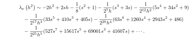
24: 28.16 Asymptotic Expansions for Large $q$

… ►

28.16.1 $${\lambda }_{\nu }\left(h^2\right)\sim -2h^2+2sh-\frac{1}{8}(s^2+1)-\frac{1}{2^{7}h}(s^3+3s)-\frac{1}{2^{12}{h}^2}(5s^4+34s^2+9)-\frac{1}{2^{17}{h}^3}(33s^5+410s^3+405s)-\frac{1}{2^{20}{h}^4}(63s^6+1260s^4+2943s^2+486)-\frac{1}{2^{25}{h}^5}(527s^7+15617s^5+69001s^3+41607s)+\mathrm{\cdots }.$$

ⓘ

Symbols:

${\lambda }_{\nu +2n}\left(q\right)$: eigenvalues of Mathieu equation, $\sim$: Poincaré asymptotic expansion, $h$: parameter and $\nu$: complex parameter

Permalink:

http://dlmf.nist.gov/28.16.E1

Encodings:

pMML, png, TeX

See also:

Annotations for §28.16 and Ch.28

…

25: 11.14 Tables

… ►

Abramowitz and Stegun (1964, Chapter 12) tabulates ${𝐇}_n\left(x\right)$, ${𝐇}_n\left(x\right)-Y_n\left(x\right)$, and $I_n\left(x\right)-{𝐋}_n\left(x\right)$ for $n=0,1$ and $x=0(.1)5$, $x^{-1}=0(.01)0.2$ to 6D or 7D.

… ►

Barrett (1964) tabulates ${𝐋}_n\left(x\right)$ for $n=0,1$ and $x=0.2(.005)4(.05)10(.1)19.2$ to 5 or 6S, $x=6(.25)59.5(.5)100$ to 2S.

… ►

Zhang and Jin (1996) tabulates ${𝐇}_n\left(x\right)$ and ${𝐋}_n\left(x\right)$ for $n=-4(1)3$ and $x=0(1)20$ to 8D or 7S.

… ►

Abramowitz and Stegun (1964, Chapter 12) tabulates ${\int }_0^x(I_0\left(t\right)-{𝐋}_0\left(t\right))dt$ and $(2/\pi ){\int }_x^{\mathrm{\infty }}{t}^{-1}{𝐇}_0\left(t\right)dt$ for $x=0(.1)5$ to 5D or 7D; ${\int }_0^x({𝐇}_0\left(t\right)-Y_0\left(t\right))dt-(2/\pi )\ln x$, ${\int }_0^x(I_0\left(t\right)-{𝐋}_0\left(t\right))dt-(2/\pi )\ln x$, and ${\int }_x^{\mathrm{\infty }}{t}^{-1}({𝐇}_0\left(t\right)-Y_0\left(t\right))dt$ for $x^{-1}=0(.01)0.2$ to 6D.

…

26: Bibliography K

… ►

On the Umemura polynomials for the Painlevé III equation. Phys. Lett. A 260 (6), pp. 462–467.

ⓘ

External Links:

ISSN 0375-9601, MathReview, ZentralBlatt

Referenced by:

§32.8(iii).

Encodings:

BibTeX

… ►

On the evaluation of the Gauss hypergeometric function. C. R. Acad. Bulgare Sci. 45 (6), pp. 35–36.

ⓘ

External Links:

ISSN 0861-1459, MathReview, ZentralBlatt

Referenced by:

§15.15, §15.19(i).

Encodings:

BibTeX

… ►

The second Painlevé equation in electric probe theory. Some numerical solutions. Zh. Vychisl. Mat. Mat. Fiz. 38 (6), pp. 992–1000 (Russian).

ⓘ

Notes:

In Russian. English translation: Comput. Math. Math. Phys. 38(1998), no. 6, pp. 950–958

External Links:

ISSN 0044-4669, MathReview, ZentralBlatt

Referenced by:

§32.17.

Encodings:

BibTeX

… ►

Calculation of the multiple zeros of the derivatives of the cylindrical Bessel functions $J_{\nu }(z)$ and $Y_{\nu }(z)$ . Zh. Vychisl. Mat. i Mat. Fiz. 25 (12), pp. 1749–1760, 1918.

ⓘ

Notes:

English translation in U.S.S.R. Computational Math. and Math. Phys. 25(6), pp. 101–107

External Links:

ISSN 0044-4669, Document, MathReview (E. Riekstiņš), ZentralBlatt

Referenced by:

§10.74(vi), 10th item.

Encodings:

BibTeX

… ►

An improvement of the remainder term in the divisor problem. Mat. Zametki 6, pp. 545–554 (Russian).

ⓘ

Notes:

In Russian. English translation: Math. Notes 6(1969), no. 5, pp. 784–791.

External Links:

Document, MathReview (A. I. Vinogradov), ZentralBlatt

Referenced by:

§27.11, Erratum (V1.1.8) for Section 27.11.

Encodings:

BibTeX

…

27: 18.8 Differential Equations

… ►6 of Abramowitz and Stegun (1964). ►

Table 18.8.1: Classical OP’s: differential equations $A(x)f^{\prime \prime }(x)+B(x)f^{\prime }(x)+C(x)f(x)+{\lambda }_{n}f(x)=0$.

► ►►►►►

#	$f(x)$	$A(x)$	$B(x)$	$C(x)$	${\lambda }_n$
…
3	${(\sin x)}^{\alpha +\frac{1}{2}}{P}_n^{(\alpha ,\alpha )}\left(\cos x\right)$	$1$	$0$	$(\frac{1}{4}-{\alpha }^2)/{\sin }^{2}x$	${(n+\alpha +\frac{1}{2})}^2$
…
6	$U_n\left(x\right)$	$1-x^2$	$-3x$	$0$	$n(n+2)$
…
12	$H_n\left(x\right)$	$1$	$-2x$	$0$	$2n$
…

►

…

28: 18.41 Tables

… ►Abramowitz and Stegun (1964, Tables 22.4, 22.6, 22.11, and 22.13) tabulates $T_n\left(x\right)$, $U_n\left(x\right)$, $L_n\left(x\right)$, and $H_n\left(x\right)$ for $n=0(1)12$. The ranges of $x$ are $0.2(.2)1$ for $T_n\left(x\right)$ and $U_n\left(x\right)$, and $0.5,1,3,5,10$ for $L_n\left(x\right)$ and $H_n\left(x\right)$. …

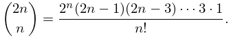
29: 26.3 Lattice Paths: Binomial Coefficients

… ► $\left(\genfrac{}{}{0.0pt}{}{m}{n}\right)$ is the number of ways of choosing $n$ objects from a collection of $m$ distinct objects without regard to order. … ►

Table 26.3.2: Binomial coefficients $\left(\genfrac{}{}{0.0pt}{}{m+n}{m}\right)$ for lattice paths.

► ►►►►►

$m$	$n$
	0	1	2	3	4	5	6	7	8
…
1	1	2	3	4	5	6	7	8	9
2	1	3	6	10	15	21	28	36	45
…

►

… ►

26.3.11 $$\left(\genfrac{}{}{0.0pt}{}{2n}{n}\right)=\frac{2^n(2n-1)(2n-3)\mathrm{\cdots }3\cdot 1}{n!}.$$

ⓘ

Symbols:

$\left(\genfrac{}{}{0.0pt}{}{m}{n}\right)$: binomial coefficient, $!$: factorial (as in $n!$) and $n$: nonnegative integer

A&S Ref:

24.1.1

Permalink:

http://dlmf.nist.gov/26.3.E11

Encodings:

pMML, png, TeX

See also:

Annotations for §26.3(iv), §26.3 and Ch.26

…

30: Staff

… ►

Nico M. Temme, Centrum Wiskunde Informatica, Chaps. 3, 6, 7, 12

… ►

Amparo Gil, Universidad de Cantabria, for Chap. 3

… ►

Javier Segura, Universidad de Cantabria, for Chap. 3

… ►

Nico M. Temme, Centrum Wiskunde & Informatica (CWI), for Chaps. 3, 6, 7, 12

…