integration by parts

SearchAdvancedHelp

(0.003 seconds)

11—20 of 77 matching pages

11: 2.10 Sums and Sequences

… ►

2.10.2 $$\sum _{j=a}^{n}f(j)={\int }_a^{n}f(x)dx+\frac{1}{2}f(a)+\frac{1}{2}f(n)-2{\int }_0^{\mathrm{\infty }}\frac{\mathrm{\Im }\left(f(a+\mathrm{i}y)\right)}{{\mathrm{e}}^{2\pi y}-1}dy+\sum _{s=1}^m\frac{B_{2s}}{(2s)!}{f}^{(2s-1)}(n)+2\frac{{(-1)}^m}{(2m)!}{\int }_0^{\mathrm{\infty }}\mathrm{\Im }\left(f^{(2m)}(n+\mathrm{i}{\vartheta }_{n}y)\right)\frac{y^{2m}dy}{{\mathrm{e}}^{2\pi y}-1},$$

ⓘ

Symbols:

$B_n$: Bernoulli numbers, $\pi$: the ratio of the circumference of a circle to its diameter, $dx$: differential of $x$ , $\mathrm{e}$: base of natural logarithm, $!$: factorial (as in $n!$), $\mathrm{\Im }$: imaginary part, $\mathrm{i}$: imaginary unit, $\int$: integral, $a$: integer, $m$: integer, $n$: integer and $f(x)$: integrable function

Referenced by:

item (c), §2.10(i)

Permalink:

http://dlmf.nist.gov/2.10.E2

Encodings:

pMML, png, TeX

See also:

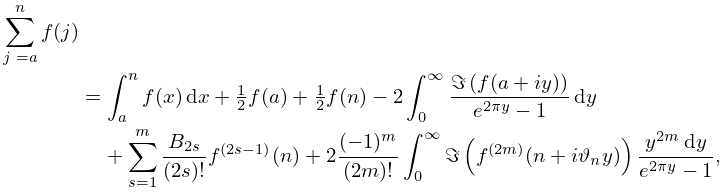
Annotations for §2.10(i), §2.10 and Ch.2

… ►This identity can be used to find asymptotic approximations for large $n$ when the factor $v_j$ changes slowly with $j$, and $u_j$ is oscillatory; compare the approximation of Fourier integrals by integration by parts in §2.3(i). … ►In these circumstances the integrals in (2.10.28) are integrable by parts $m$ times, yielding …

12: 5.9 Integral Representations

… ►

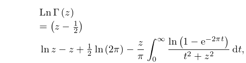
5.9.10_1 $$\mathrm{Ln}\mathrm{\Gamma }\left(z\right)=\left(z-\frac{1}{2}\right)\ln z-z+\frac{1}{2}\ln \left(2\pi \right)-\frac{z}{\pi }{\int }_0^{\mathrm{\infty }}\frac{\ln \left(1-{\mathrm{e}}^{-2\pi t}\right)}{t^2+z^2}dt,$$

ⓘ

Symbols:

$\mathrm{\Gamma }\left(z\right)$: gamma function, $\pi$: the ratio of the circumference of a circle to its diameter, $dx$: differential of $x$ , $\mathrm{e}$: base of natural logarithm, $\int$: integral, $\mathrm{Ln}z$: general logarithm function, $\ln z$: principal branch of logarithm function and $z$: complex variable

Proof sketch:

Can be obtained from (5.9.10) via integration by parts.

Referenced by:

§5.9(i), Erratum (V1.1.7) for Additions

Permalink:

http://dlmf.nist.gov/5.9.E10_1

Encodings:

pMML, png, TeX

Addition (effective with 1.1.7):

This equation was added.

See also:

Annotations for §5.9(i), §5.9(i), §5.9 and Ch.5

…

13: 2.11 Remainder Terms; Stokes Phenomenon

… ►By integration by parts (§2.3(i)) …

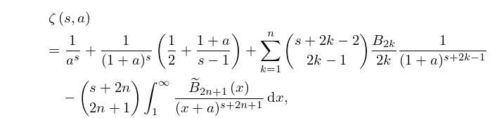
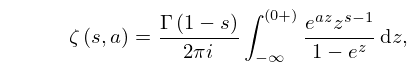
14: 25.11 Hurwitz Zeta Function

… ►

25.11.7 $$\zeta (s,a)=\frac{1}{a^s}+\frac{1}{{(1+a)}^s}\left(\frac{1}{2}+\frac{1+a}{s-1}\right)+\sum _{k=1}^n\left(\genfrac{}{}{0.0pt}{}{s+2k-2}{2k-1}\right)\frac{B_{2k}}{2k}\frac{1}{{(1+a)}^{s+2k-1}}-\left(\genfrac{}{}{0.0pt}{}{s+2n}{2n+1}\right){\int }_1^{\mathrm{\infty }}\frac{{\tilde{B}}_{2n+1}\left(x\right)}{{(x+a)}^{s+2n+1}}dx,$$ $s\ne 1$, $a>0$, $n=1,2,3,\mathrm{\dots }$, $\mathrm{\Re }s>-2n$.

ⓘ

Symbols:

$B_n$: Bernoulli numbers, $\zeta (s,a)$: Hurwitz zeta function, $\left(\genfrac{}{}{0.0pt}{}{m}{n}\right)$: binomial coefficient, $dx$: differential of $x$ , $\int$: integral, ${\tilde{B}}_n\left(x\right)$: periodic Bernoulli functions, $\mathrm{\Re }$: real part, $k$: nonnegative integer, $n$: nonnegative integer, $x$: real variable, $a$: real or complex parameter and $s$: complex variable

Keywords:

Euler–Maclaurin formula, improper integral

Proof sketch:

Derivable from (25.11.5) by setting $N=1$ and repeatedly integrating by parts using (1.2.6), (24.2.2), (24.2.4), (24.2.11), (24.2.12), (24.4.34).

Permalink:

http://dlmf.nist.gov/25.11.E7

Encodings:

pMML, png, TeX

See also:

Annotations for §25.11(iii), §25.11 and Ch.25

… ►

25.11.30 $$\zeta (s,a)=\frac{\mathrm{\Gamma }\left(1-s\right)}{2\pi \mathrm{i}}{\int }_{-\mathrm{\infty }}^{(0+)}\frac{{\mathrm{e}}^{az}{z}^{s-1}}{1-{\mathrm{e}}^z}dz,$$ $s\ne 1$, $\mathrm{\Re }a>0$,

ⓘ

Symbols:

$\mathrm{\Gamma }\left(z\right)$: gamma function, $\zeta (s,a)$: Hurwitz zeta function, $\pi$: the ratio of the circumference of a circle to its diameter, $dx$: differential of $x$ , $\mathrm{e}$: base of natural logarithm, $\mathrm{i}$: imaginary unit, $\int$: integral, $\mathrm{\Re }$: real part, $a$: real or complex parameter, $s$: complex variable and $z$: complex variable

Keywords:

contour integral, integral representation

Source:

Erdélyi et al. (1953a, (1.10.5), p. 25); with $z=-t$

Proof sketch:

This contour integral uses Hankel’s contour Figure 5.9.1. Assume $\mathrm{\Re }s>1$, collapse the integration path onto the negative real axis, apply (25.11.25), followed by analytic continuation for all $s\ne 1$, $\mathrm{\Re }a>0$, since the integrand is analytic in $z$, the convergence at the ends of the path is exponential for all $s\ne -1$ and the Hankel contour can be kept well clear of the singularity at the origin in the $z$-plane.

Referenced by:

§25.11(i)

Permalink:

http://dlmf.nist.gov/25.11.E30

Encodings:

pMML, png, TeX

See also:

Annotations for §25.11(vii), §25.11 and Ch.25

…

15: 18.18 Sums

… ►

Expansion of $L^2$ functions

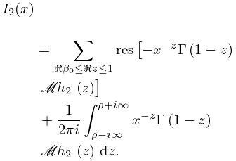
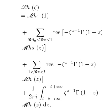
►In all three cases of Jacobi, Laguerre and Hermite, if $f(x)$ is $L^2$ on the corresponding interval with respect to the corresponding weight function and if $a_n,b_n,d_n$ are given by (18.18.1), (18.18.5), (18.18.7), respectively, then the respective series expansions (18.18.2), (18.18.4), (18.18.6) are valid with the sums converging in $L^2$ sense. … ►See (18.17.45) and (18.17.49) for integrated forms of (18.18.22) and (18.18.23), respectively. …

16: 2.5 Mellin Transform Methods

… ►

2.5.6

ⓘ

Symbols:

$ℳ\left(f\right)\left(s\right)$: Mellin transform, $\mathrm{\Re }$: real part, $res$: residue, $f(x)$: locally integrable function, $c$: point, $I(x)$: convolution integral, $h(x)$: function, $d$: point and $E(x)$: function

Keywords:

Mellin transform

Referenced by:

§2.5(i), §2.5(i)

Permalink:

http://dlmf.nist.gov/2.5.E6

Encodings:

pMML, png, TeX

Notational Change (effective with 1.0.15):

The notation for the Mellin transform was changed to $ℳf\left(z\right)$ from $ℳ(f;z)$.

See also:

Annotations for §2.5(i), §2.5 and Ch.2

… ►

2.5.42 $$I_2(x)=\sum _{\mathrm{\Re }{\beta }_0\le \mathrm{\Re }z\le 1}res\left[-x^{-z}\mathrm{\Gamma }\left(1-z\right)ℳh_2\left(z\right)\right]+\frac{1}{2\pi \mathrm{i}}{\int }_{\rho -\mathrm{i}\mathrm{\infty }}^{\rho +\mathrm{i}\mathrm{\infty }}{x}^{-z}\mathrm{\Gamma }\left(1-z\right)ℳh_2\left(z\right)dz.$$

ⓘ

Symbols:

$\mathrm{\Gamma }\left(z\right)$: gamma function, $ℳ\left(f\right)\left(s\right)$: Mellin transform, $\pi$: the ratio of the circumference of a circle to its diameter, $dx$: differential of $x$ , $\mathrm{i}$: imaginary unit, $\int$: integral, $\mathrm{\Re }$: real part, $res$: residue, $h(x)$: locally integrable function, $I_j(x)$: integral and $\rho$: parameter

Keywords:

Mellin transform

Referenced by:

§2.5(iii)

Permalink:

http://dlmf.nist.gov/2.5.E42

Encodings:

pMML, png, TeX

Notational Change (effective with 1.0.15):

The notation for the Mellin transform was changed to $ℳf\left(z\right)$ from $ℳ(f;z)$.

See also:

Annotations for §2.5(iii), §2.5 and Ch.2

… ►

2.5.43

ⓘ

Symbols:

$\mathrm{\Gamma }\left(z\right)$: gamma function, $ℒ\left(f\right)\left(s\right)$: Laplace transform, $ℳ\left(f\right)\left(s\right)$: Mellin transform, $\pi$: the ratio of the circumference of a circle to its diameter, $dx$: differential of $x$ , $\mathrm{i}$: imaginary unit, $\int$: integral, $\mathrm{\Re }$: real part, $res$: residue, $h(x)$: locally integrable function and $\delta$: arbitrary small positive constant

Keywords:

Laplace transform, Mellin transform

Referenced by:

§2.5(iii), §2.5(iii)

Permalink:

http://dlmf.nist.gov/2.5.E43

Encodings:

pMML, png, TeX

Notational Change (effective with 1.0.15):

The notation for the Laplace transform was changed to $ℒf\left(z\right)$ from $ℒ(f;z)$. In addition, the notation for the Mellin transform was changed to $ℳf\left(z\right)$ from $ℳ(f;z)$.

See also:

Annotations for §2.5(iii), §2.5 and Ch.2

… ►

2.5.45 $$ℒh\left(\zeta \right)={\int }_0^{\mathrm{\infty }}\frac{{\mathrm{e}}^{-\zeta t}}{1+t}dt,$$ $\mathrm{\Re }\zeta >0$.

ⓘ

Symbols:

$ℒ\left(f\right)\left(s\right)$: Laplace transform, $dx$: differential of $x$ , $\mathrm{e}$: base of natural logarithm, $\int$: integral, $\mathrm{\Re }$: real part and $h(x)$: locally integrable function

Keywords:

Laplace transform

Permalink:

http://dlmf.nist.gov/2.5.E45

Encodings:

pMML, png, TeX

Notational Change (effective with 1.0.15):

The notation for the Laplace transform was changed to $ℒf\left(z\right)$ from $ℒ(f;z)$.

See also:

Annotations for §2.5(iii), §2.5(iii), §2.5 and Ch.2

…

17: 21.9 Integrable Equations

… ►Riemann theta functions arise in the study of integrable differential equations that have applications in many areas, including fluid mechanics (Ablowitz and Segur (1981, Chapter 4)), magnetic monopoles (Ercolani and Sinha (1989)), and string theory (Deligne et al. (1999, Part 3)). …

18: 1.18 Linear Second Order Differential Operators and Eigenfunction Expansions

… ►We integrate by parts twice giving: …

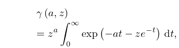
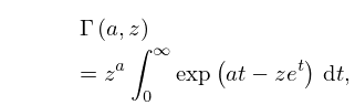
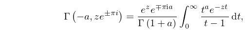
19: 8.6 Integral Representations

… ►

8.6.3 $$\gamma (a,z)=z^a{\int }_0^{\mathrm{\infty }}\exp \left(-at-z{\mathrm{e}}^{-t}\right)dt,$$ $\mathrm{\Re }a>0$.

ⓘ

Symbols:

$dx$: differential of $x$ , $\exp z$: exponential function, $\mathrm{e}$: base of natural logarithm, $\gamma (a,z)$: incomplete gamma function, $\int$: integral, $\mathrm{\Re }$: real part, $z$: complex variable and $a$: parameter

Referenced by:

§8.6(i)

Permalink:

http://dlmf.nist.gov/8.6.E3

Encodings:

pMML, png, TeX

See also:

Annotations for §8.6(i), §8.6 and Ch.8

… ►

8.6.7 $$\mathrm{\Gamma }(a,z)=z^a{\int }_0^{\mathrm{\infty }}\exp \left(at-z{\mathrm{e}}^t\right)dt,$$ $\mathrm{\Re }z>0$.

ⓘ

Symbols:

$dx$: differential of $x$ , $\exp z$: exponential function, $\mathrm{e}$: base of natural logarithm, $\mathrm{\Gamma }(a,z)$: incomplete gamma function, $\int$: integral, $\mathrm{\Re }$: real part, $z$: complex variable and $a$: parameter

Referenced by:

§8.6(i)

Permalink:

http://dlmf.nist.gov/8.6.E7

Encodings:

pMML, png, TeX

See also:

Annotations for §8.6(i), §8.6 and Ch.8

… ►

8.6.9 $$\mathrm{\Gamma }(-a,z{\mathrm{e}}^{\pm \pi \mathrm{i}})=\frac{{\mathrm{e}}^z{\mathrm{e}}^{\mp \pi \mathrm{i}a}}{\mathrm{\Gamma }\left(1+a\right)}{\int }_0^{\mathrm{\infty }}\frac{t^a{\mathrm{e}}^{-zt}}{t-1}dt,$$ $\mathrm{\Re }z>0$, $\mathrm{\Re }a>-1$,

ⓘ

Symbols:

$\mathrm{\Gamma }\left(z\right)$: gamma function, $\pi$: the ratio of the circumference of a circle to its diameter, $dx$: differential of $x$ , $\mathrm{e}$: base of natural logarithm, $\mathrm{i}$: imaginary unit, $\mathrm{\Gamma }(a,z)$: incomplete gamma function, $\int$: integral, $\mathrm{\Re }$: real part, $z$: complex variable and $a$: parameter

Referenced by:

§8.6(ii)

Permalink:

http://dlmf.nist.gov/8.6.E9

Encodings:

pMML, png, TeX

See also:

Annotations for §8.6(ii), §8.6 and Ch.8

►where the integration path passes above or below the pole at $t=1$, according as upper or lower signs are taken. … ►In (8.6.10)–(8.6.12), $c$ is a real constant and the path of integration is indented (if necessary) so that in the case of (8.6.10) it separates the poles of the gamma function from the pole at $s=a$, in the case of (8.6.11) it is to the right of all poles, and in the case of (8.6.12) it separates the poles of the gamma function from the poles at $s=0,1,2,\mathrm{\dots }$. …

20: 4.38 Inverse Hyperbolic Functions: Further Properties

… ►

4.38.2 $$\mathrm{arcsinh}z=\ln \left(2z\right)+\frac{1}{2}\frac{1}{2z^2}-\frac{1\cdot 3}{2\cdot 4}\frac{1}{4z^4}+\frac{1\cdot 3\cdot 5}{2\cdot 4\cdot 6}\frac{1}{6z^6}-\mathrm{\cdots },$$ $\mathrm{\Re }z>0$, $|z|>1$.

ⓘ

Symbols:

$\mathrm{arcsinh}z$: inverse hyperbolic sine function, $\ln z$: principal branch of logarithm function, $\mathrm{\Re }$: real part and $z$: complex variable

A&S Ref:

4.6.31 (misses a condition on $z$.)

Referenced by:

§4.38(i)

Permalink:

http://dlmf.nist.gov/4.38.E2

Encodings:

pMML, png, TeX

See also:

Annotations for §4.38(i), §4.38 and Ch.4

… ►

4.38.4 $$\mathrm{arccosh}z={(2(z-1))}^{1/2}\left(1+\sum _{n=1}^{\mathrm{\infty }}{(-1)}^n\frac{1\cdot 3\cdot 5\mathrm{\cdots }(2n-1)}{2^{2n}n!(2n+1)}{(z-1)}^n\right),$$ $\mathrm{\Re }z>0$, $|z-1|\le 2$.

ⓘ

Symbols:

$!$: factorial (as in $n!$), $\mathrm{arccosh}z$: inverse hyperbolic cosine function, $\mathrm{\Re }$: real part, $n$: integer and $z$: complex variable

Referenced by:

§4.38(i)

Permalink:

http://dlmf.nist.gov/4.38.E4

Encodings:

pMML, png, TeX

See also:

Annotations for §4.38(i), §4.38 and Ch.4

… ►

4.38.7 $$\mathrm{arctanh}z=\frac{z}{1-z^2}\left(1+\frac{2}{3}\frac{z^2}{z^2-1}+\frac{2\cdot 4}{3\cdot 5}{\left(\frac{z^2}{z^2-1}\right)}^2+\mathrm{\cdots }\right),$$ ,

ⓘ

Symbols:

$\mathrm{arctanh}z$: inverse hyperbolic tangent function, $\mathrm{\Re }$: real part and $z$: complex variable

Referenced by:

§4.38(i)

Permalink:

http://dlmf.nist.gov/4.38.E7

Encodings:

pMML, png, TeX

See also:

Annotations for §4.38(i), §4.38 and Ch.4

… ►

4.38.10 $$\frac{d}{dz}\mathrm{arccosh}z=\pm {(z^2-1)}^{-1/2},$$ $\mathrm{\Re }z\gtrless 0$.

ⓘ

Symbols:

$\frac{df}{dx}$: derivative of $f$ with respect to $x$ , $\mathrm{arccosh}z$: inverse hyperbolic cosine function, $\mathrm{\Re }$: real part and $z$: complex variable

A&S Ref:

4.6.38 (has an error.)

Permalink:

http://dlmf.nist.gov/4.38.E10

Encodings:

pMML, png, TeX

See also:

Annotations for §4.38(ii), §4.38 and Ch.4

… ►

4.38.12 $$\frac{d}{dz}\mathrm{arccsch}z=\mp \frac{1}{z{(1+z^2)}^{1/2}},$$ $\mathrm{\Re }z\gtrless 0$.

ⓘ

Symbols:

$\frac{df}{dx}$: derivative of $f$ with respect to $x$ , $\mathrm{arccsch}z$: inverse hyperbolic cosecant function, $\mathrm{\Re }$: real part and $z$: complex variable

A&S Ref:

4.6.40

Permalink:

http://dlmf.nist.gov/4.38.E12

Encodings:

pMML, png, TeX

See also:

Annotations for §4.38(ii), §4.38 and Ch.4

…