Whipple 3F2 sum
(0.002 seconds)
11—20 of 660 matching pages
11: 34.5 Basic Properties: Symbol
…
►Examples are provided by:
…
►
§34.5(vi) Sums
… ►Equations (34.5.15) and (34.5.16) are the sum rules. They constitute addition theorems for the symbol. … ►For other sums see Ginocchio (1991).12: 34.3 Basic Properties: Symbol
§34.3 Basic Properties: Symbol
… ►§34.3(ii) Symmetry
… ►§34.3(iv) Orthogonality
… ►§34.3(vi) Sums
►For sums of products of symbols, see Varshalovich et al. (1988, pp. 259–262). …13: 34.4 Definition: Symbol
§34.4 Definition: Symbol
►The symbol is defined by the following double sum of products of symbols: … ►Except in degenerate cases the combination of the triangle inequalities for the four symbols in (34.4.1) is equivalent to the existence of a tetrahedron (possibly degenerate) with edges of lengths ; see Figure 34.4.1. … ►The symbol can be expressed as the finite sum … ►For alternative expressions for the symbol, written either as a finite sum or as other terminating generalized hypergeometric series of unit argument, see Varshalovich et al. (1988, §§9.2.1, 9.2.3).14: 5.16 Sums
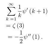
§5.16 Sums
… ►
5.16.2
►For further sums involving the psi function see Hansen (1975, pp. 360–367).
For sums of gamma functions see Andrews et al. (1999, Chapters 2 and 3) and §§15.2(i), 16.2.
►For related sums involving finite field analogs of the gamma and beta functions (Gauss and Jacobi sums) see Andrews et al. (1999, Chapter 1) and Terras (1999, pp. 90, 149).
15: 34.13 Methods of Computation
§34.13 Methods of Computation
►Methods of computation for and symbols include recursion relations, see Schulten and Gordon (1975a), Luscombe and Luban (1998), and Edmonds (1974, pp. 42–45, 48–51, 97–99); summation of single-sum expressions for these symbols, see Varshalovich et al. (1988, §§8.2.6, 9.2.1) and Fang and Shriner (1992); evaluation of the generalized hypergeometric functions of unit argument that represent these symbols, see Srinivasa Rao and Venkatesh (1978) and Srinivasa Rao (1981). ►For symbols, methods include evaluation of the single-sum series (34.6.2), see Fang and Shriner (1992); evaluation of triple-sum series, see Varshalovich et al. (1988, §10.2.1) and Srinivasa Rao et al. (1989). …16: 34.9 Graphical Method
§34.9 Graphical Method
… ►For specific examples of the graphical method of representing sums involving the , and symbols, see Varshalovich et al. (1988, Chapters 11, 12) and Lehman and O’Connell (1973, §3.3).17: 23.9 Laurent and Other Power Series
…
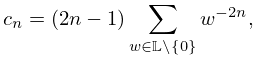
►
►
23.9.1
.
…
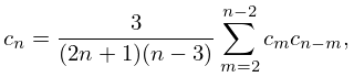
►
23.9.5
.
►Explicit coefficients in terms of and are given up to in Abramowitz and Stegun (1964, p. 636).
►For , and with as in §23.3(i),
…
18: 34.6 Definition: Symbol
…
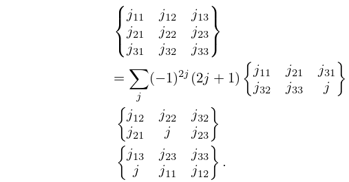
►The symbol may be defined either in terms of symbols or equivalently in terms of symbols:
►
34.6.1
►
34.6.2
►The symbol may also be written as a finite triple sum equivalent to a terminating generalized hypergeometric series of three variables with unit arguments.
…
19: 10.19 Asymptotic Expansions for Large Order
…
►In these expansions and are the polynomials in of degree defined in §10.41(ii).
…
►with sectors of validity .
…
►
,
►
.
…
►with sectors of validity and , respectively.
…
