Whipple 3F2 sum

SearchAdvancedHelp

(0.003 seconds)

1—10 of 660 matching pages

1: 34.2 Definition: $\mathit{3}j$ Symbol

§34.2 Definition: $\mathit{3}j$ Symbol

… ►The corresponding projective quantum numbers $m_1,m_2,m_3$ are given by … ►When both conditions are satisfied the $\mathit{3}j$ symbol can be expressed as the finite sum … ►where ${}_3{}^{}F_2^{}$ is defined as in §16.2. ►For alternative expressions for the $\mathit{3}j$ symbol, written either as a finite sum or as other terminating generalized hypergeometric series ${}_3{}^{}F_2^{}$ of unit argument, see Varshalovich et al. (1988, §§8.21, 8.24–8.26).

2: 14.19 Toroidal (or Ring) Functions

… ►

14.19.2 $$P_{\nu -\frac{1}{2}}^{\mu }\left(\cosh \xi \right)=\frac{\mathrm{\Gamma }\left(\frac{1}{2}-\mu \right)}{{\pi }^{1/2}{\left(1-{\mathrm{e}}^{-2\xi }\right)}^{\mu }{\mathrm{e}}^{(\nu +(1/2))\xi }}𝐅(\frac{1}{2}-\mu ,\frac{1}{2}+\nu -\mu ;1-2\mu ;1-{\mathrm{e}}^{-2\xi }),$$ $\mu \ne \frac{1}{2},\frac{3}{2},\frac{5}{2},\mathrm{\dots }$.

ⓘ

Symbols:

$\mathrm{\Gamma }\left(z\right)$: gamma function, $P_{\nu }^{\mu }\left(z\right)$: associated Legendre function of the first kind, $\pi$: the ratio of the circumference of a circle to its diameter, $\mathrm{e}$: base of natural logarithm, $\cosh z$: hyperbolic cosine function, $𝐅(a,b;c;z)$ or $𝐅(\genfrac{}{}{0pt}{}{a,b}{c};z)$: $={}_2{}^{}𝐅_1^{}(a,b;c;z)$ Olver’s hypergeometric function, $\mu$: general order, $\nu$: general degree and $\xi >0$: variable

Referenced by:

§14.19(ii), Erratum (V1.0.1) for Equation (14.19.2)

Permalink:

http://dlmf.nist.gov/14.19.E2

Encodings:

pMML, png, TeX

Errata (effective with 1.0.1):

Originally the argument to $𝐅$ was incorrect and the condition on $\mu$ too weak:

$$P_{\nu -\frac{1}{2}}^{\mu }\left(\cosh \xi \right)=\frac{\mathrm{\Gamma }\left(1-2\mu \right)2^{2\mu }}{\mathrm{\Gamma }\left(1-\mu \right){\left(1-{\mathrm{e}}^{-2\xi }\right)}^{\mu }{\mathrm{e}}^{(\nu +(1/2))\xi }}𝐅(\frac{1}{2}-\mu ,\frac{1}{2}+\nu -\mu ;1-2\mu ;{\mathrm{e}}^{-2\xi }),$$ $\mu \ne \frac{1}{2}$.

Also, the factor multiplying $𝐅$ was rewritten to clarify the poles, which determine the correct condition on $\mu$.

Reported 2010-11-02 by Alvaro Valenzuela

See also:

Annotations for §14.19(ii), §14.19 and Ch.14

… ►

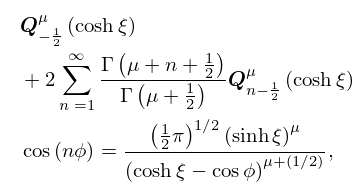
§14.19(iv) Sums

… ►

14.19.6 $${𝑸}_{-\frac{1}{2}}^{\mu }\left(\cosh \xi \right)+2\sum _{n=1}^{\mathrm{\infty }}\frac{\mathrm{\Gamma }\left(\mu +n+\frac{1}{2}\right)}{\mathrm{\Gamma }\left(\mu +\frac{1}{2}\right)}{𝑸}_{n-\frac{1}{2}}^{\mu }\left(\cosh \xi \right)\cos \left(n\varphi \right)=\frac{{\left(\frac{1}{2}\pi \right)}^{1/2}{\left(\sinh \xi \right)}^{\mu }}{{\left(\cosh \xi -\cos \varphi \right)}^{\mu +(1/2)}},$$ $\mathrm{\Re }\mu >-\frac{1}{2}$.

ⓘ

Symbols:

$\mathrm{\Gamma }\left(z\right)$: gamma function, ${𝑸}_{\nu }^{\mu }\left(z\right)$: Olver’s associated Legendre function, $\pi$: the ratio of the circumference of a circle to its diameter, $\cos z$: cosine function, $\cosh z$: hyperbolic cosine function, $\sinh z$: hyperbolic sine function, $\mathrm{\Re }$: real part, $n$: nonnegative integer, $\mu$: general order and $\xi >0$: variable

Permalink:

http://dlmf.nist.gov/14.19.E6

Encodings:

pMML, png, TeX

See also:

Annotations for §14.19(iv), §14.19 and Ch.14

►

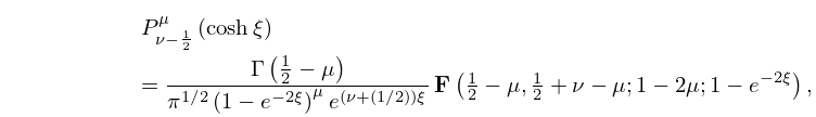
§14.19(v) Whipple’s Formula for Toroidal Functions

…

3: 16.4 Argument Unity

… ►

Lerch Sum

… ►

Watson’s Sum

… ►

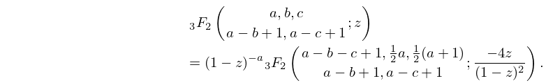
Whipple’s Sum

… ►

Džrbasjan’s Sum

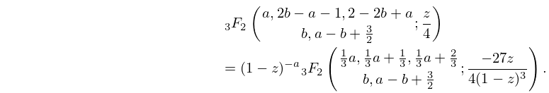
… ►A different type of transformation is that of Whipple: …

4: 16.6 Transformations of Variable

… ►

16.6.1 $${}_3{}^{}F_2^{}(\genfrac{}{}{0pt}{}{a,b,c}{a-b+1,a-c+1};z)={(1-z)}^{-a}{}_3{}^{}F_2^{}(\genfrac{}{}{0pt}{}{a-b-c+1,\frac{1}{2}a,\frac{1}{2}(a+1)}{a-b+1,a-c+1};\frac{-4z}{{(1-z)}^2}).$$

ⓘ

Symbols:

${}_p{}^{}F_q^{}(a_1,\mathrm{\dots },a_p;b_1,\mathrm{\dots },b_q;z)$ or ${}_p{}^{}F_q^{}(\genfrac{}{}{0pt}{}{a_1,\mathrm{\dots },a_p}{b_1,\mathrm{\dots },b_q};z)$: alternatively ${}_p{}^{}F_q^{}(𝐚;𝐛;z)$ or ${}_p{}^{}F_q^{}(\genfrac{}{}{0pt}{}{𝐚}{𝐛};z)$
generalized hypergeometric function, $z$: complex variable, $a,a_1,\mathrm{\dots },a_p$: real or complex parameters and $b,b_1,\mathrm{\dots },b_q$: real or complex parameters

Referenced by:

§16.6

Permalink:

http://dlmf.nist.gov/16.6.E1

Encodings:

pMML, png, TeX

See also:

Annotations for §16.6, §16.6 and Ch.16

… ►

16.6.2 $${}_3{}^{}F_2^{}(\genfrac{}{}{0pt}{}{a,2b-a-1,2-2b+a}{b,a-b+\frac{3}{2}};\frac{z}{4})={(1-z)}^{-a}{}_3{}^{}F_2^{}(\genfrac{}{}{0pt}{}{\frac{1}{3}a,\frac{1}{3}a+\frac{1}{3},\frac{1}{3}a+\frac{2}{3}}{b,a-b+\frac{3}{2}};\frac{-27z}{4{(1-z)}^3}).$$

ⓘ

Symbols:

${}_p{}^{}F_q^{}(a_1,\mathrm{\dots },a_p;b_1,\mathrm{\dots },b_q;z)$ or ${}_p{}^{}F_q^{}(\genfrac{}{}{0pt}{}{a_1,\mathrm{\dots },a_p}{b_1,\mathrm{\dots },b_q};z)$: alternatively ${}_p{}^{}F_q^{}(𝐚;𝐛;z)$ or ${}_p{}^{}F_q^{}(\genfrac{}{}{0pt}{}{𝐚}{𝐛};z)$
generalized hypergeometric function, $z$: complex variable, $a,a_1,\mathrm{\dots },a_p$: real or complex parameters and $b,b_1,\mathrm{\dots },b_q$: real or complex parameters

Referenced by:

§16.6

Permalink:

http://dlmf.nist.gov/16.6.E2

Encodings:

pMML, png, TeX

See also:

Annotations for §16.6, §16.6 and Ch.16

…

5: Bibliography W

… ►

Extension of a quadratic transformation due to Whipple with an application. Adv. Difference Equ., pp. 2013:157, 8.

ⓘ

External Links:

ISSN 1687-1847, Document, FullText, MathReview (Daniele Ritelli), ZentralBlatt

Referenced by:

§16.6, §16.6.

Encodings:

BibTeX

… ►

Surface Waves. In Handbuch der Physik, Vol. 9, Part 3, pp. 446–778.

ⓘ

External Links:

Online edition, MathReview (F. Ursell), ZentralBlatt

Referenced by:

§11.12.

Encodings:

BibTeX

… ►

Harmonic Analysis. In Studies in Real and Complex Analysis, I. I. Hirschman (Ed.), Studies in Mathematics, Vol. 3, pp. 124–178.

ⓘ

External Links:

MathReview, ZentralBlatt

Referenced by:

§1.15(iii), §1.15(iv), §1.15(v).

Encodings:

BibTeX

… ►

Some transformations of generalized hypergeometric series. Proc. London Math. Soc. (2) 26 (2), pp. 257–272.

ⓘ

External Links:

Document, ZentralBlatt

Referenced by:

§16.6.

Encodings:

BibTeX

… ►

Asymptotics for the ${}_4{}^{}F_3^{}$ polynomials. J. Approx. Theory 66 (1), pp. 58–71.

ⓘ

External Links:

ISSN 0021-9045, Document, MathReview (R. G. Buschman), ZentralBlatt

Referenced by:

§18.26(v).

Encodings:

BibTeX

…

6: 17.9 Further Transformations of ${}_{r+1}{}^{}\varphi _r^{}$ Functions

… ►

§17.9(ii) ${}_3{}^{}\varphi _2^{}\to {}_3{}^{}\varphi _2^{}$

►

Transformations of ${}_3{}^{}\varphi _2^{}$-Series

… ►

Sears’ Balanced ${}_4{}^{}\varphi _3^{}$ Transformations

… ►

Watson’s $q$-Analog of Whipple’s Theorem

… ►

§17.9(iv) Bibasic Series

…

7: 17.7 Special Cases of Higher ${}_r{}^{}\varphi _s^{}$ Functions

… ►

$q$-Analog of Dixon’s ${}_3{}^{}F_2^{}\left(1\right)$ Sum

… ►

Gasper–Rahman $q$-Analog of Watson’s ${}_3{}^{}F_2^{}$ Sum

… ►

Gasper–Rahman $q$-Analog of Whipple’s ${}_3{}^{}F_2^{}$ Sum

… ►

Andrews’ $q$-Analog of the Terminating Version of Whipple’s ${}_3{}^{}F_2^{}$ Sum (16.4.7)

… ►

Second $q$-Analog of Bailey’s ${}_4{}^{}F_3^{}\left(1\right)$ Sum

…

8: 14.9 Connection Formulas

… ►

§14.9(iv) Whipple’s Formula

…

9: Bibliography M

… ►

On the interval computation of elementary functions. C. R. Acad. Bulgare Sci. 34 (3), pp. 319–322.

ⓘ

External Links:

ISSN 0366-8681, MathReview (David F. Griffiths), ZentralBlatt

Referenced by:

§4.45(i).

Encodings:

BibTeX

… ►

Recursion relations for the $3$-$j$ symbols. Nuclear Physics A 113 (1), pp. 215–220.

ⓘ

External Links:

Document

Referenced by:

§34.3(iii).

Encodings:

BibTeX

… ►

On the convergence of the Chebyshev series for functions possessing a singularity in the range of representation. SIAM J. Numer. Anal. 3 (3), pp. 390–409.

ⓘ

External Links:

ISSN 1095-7170, Document, MathReview (Y. L. Luke), ZentralBlatt

Referenced by:

§3.11(ii).

Encodings:

BibTeX

… ►

A $q$-analog of a Whipple’s transformation for hypergeometric series in $U(n)$ . Adv. Math. 108 (1), pp. 1–76.

ⓘ

External Links:

ISSN 0001-8708, Document, MathReview, ZentralBlatt

Referenced by:

§17.15.

Encodings:

BibTeX

… ►

Analytic Inequalities. Springer-Verlag, New York.

ⓘ

Notes:

Addenda: Univ. Beograd. Publ. Elektrotehn. Fak. Ser. Mat. Fiz., no. 634–677 (1979), pp. 3–24 and no. 577-598 (1977), pp. 3–10.

External Links:

MathReview (R. A. Askey and R. P. Boas, Jr.), ZentralBlatt

Referenced by:

§4.18, §4.32, §4.5(i), §4.5(ii), §7.8.

Encodings:

BibTeX

…

10: Errata

… ►

18.38.3 $$\sum _{m=0}^n{P}_m^{(\alpha ,0)}\left(x\right)=\frac{{\left(\alpha +2\right)}_n}{n!}{}_3{}^{}F_2^{}(\genfrac{}{}{0pt}{}{-n,n+\alpha +2,\frac{1}{2}(\alpha +1)}{\alpha +1,\frac{1}{2}(\alpha +3)};\frac{1}{2}(1-x))\ge 0,$$ $x\ge -1$, $\alpha \ge -2$, $n=0,1,\mathrm{\dots }$

This equation was updated to include the value of the sum in terms of the ${}_3{}^{}F_2^{}$ function. Also the constraint was previously $-1\le x\le 1$, $\alpha >-1$.

… ►

The title of the paragraph which was previously “Andrews’ Terminating $q$-Analog of (17.7.8)” has been changed to “Andrews’ $q$-Analog of the Terminating Version of Watson’s ${}_3{}^{}F_2^{}$ Sum (16.4.6)”. The title of the paragraph which was previously “Andrews’ Terminating $q$-Analog” has been changed to “Andrews’ $q$-Analog of the Terminating Version of Whipple’s ${}_3{}^{}F_2^{}$ Sum (16.4.7)”.

… ►

22.9.8 $$s_{1,3}^{(4)}{s}_{2,3}^{(4)}+s_{2,3}^{(4)}{s}_{3,3}^{(4)}+s_{3,3}^{(4)}{s}_{1,3}^{(4)}=\frac{{\kappa }^2-1}{k^2}$$

22.9.9 $$c_{1,3}^{(4)}{c}_{2,3}^{(4)}+c_{2,3}^{(4)}{c}_{3,3}^{(4)}+c_{3,3}^{(4)}{c}_{1,3}^{(4)}=-\frac{\kappa (\kappa +2)}{{(1+\kappa )}^2}$$

22.9.10 $$d_{1,3}^{(2)}{d}_{2,3}^{(2)}+d_{2,3}^{(2)}{d}_{3,3}^{(2)}+d_{3,3}^{(2)}{d}_{1,3}^{(2)}=d_{1,3}^{(4)}{d}_{2,3}^{(4)}+d_{2,3}^{(4)}{d}_{3,3}^{(4)}+d_{3,3}^{(4)}{d}_{1,3}^{(4)}=\kappa (\kappa +2)$$

Originally all the functions $s_{m,p}^{(4)}$, $c_{m,p}^{(4)}$ , $d_{m,p}^{(2)}$ and $d_{m,p}^{(4)}$ in Equations (22.9.8), (22.9.9) and (22.9.10) were written incorrectly with $p=2$. These functions have been corrected so that they are written with $p=3$. In the sentence just below (22.9.10), the expression $s_{m,2}^{(4)}{s}_{n,2}^{(4)}$ has been corrected to read $s_{m,p}^{(4)}{s}_{n,p}^{(4)}$.

Reported by Juan Miguel Nieto on 2019-11-07

… ►

34.3.7

In the original equation the prefactor of the above 3j symbol read ${(-1)}^{-j_2+j_3+m_3}$. It is now replaced by its correct value ${(-1)}^{j_1-j_2-m_3}$.

Reported 2014-06-12 by James Zibin.

… ►

34.4.2

Originally the factor $\mathrm{\Delta }(j_1{j}_2{j}_3)\mathrm{\Delta }(j_1{l}_2{l}_3)\mathrm{\Delta }(l_1{j}_2{l}_3)\mathrm{\Delta }(l_1{l}_2{j}_3)$ was missing in this equation.

Reported 2012-12-31 by Yu Lin.

…