§1.15 Summability Methods
Contents
- §1.15(i) Definitions for Series
- §1.15(ii) Regularity
- §1.15(iii) Summability of Fourier Series
- §1.15(iv) Definitions for Integrals
- §1.15(v) Summability of Fourier Integrals
- §1.15(vi) Fractional Integrals
- §1.15(vii) Fractional Derivatives
- §1.15(viii) Tauberian Theorems
§1.15(i) Definitions for Series
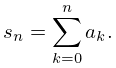
| 1.15.1 | |||
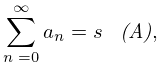
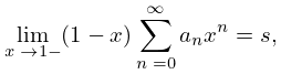
Abel Summability
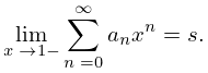
| 1.15.2 | |||
if
| 1.15.3 | |||
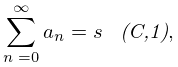
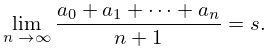
Cesàro Summability
| 1.15.4 | |||
if
| 1.15.5 | |||
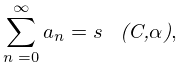
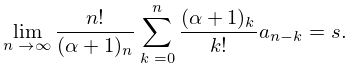
General Cesàro Summability
For ,
| 1.15.6 | |||
if
| 1.15.7 | |||
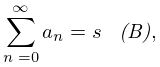
Borel Summability
| 1.15.8 | |||
if
| 1.15.9 | |||
§1.15(ii) Regularity
Methods of summation are regular if they are consistent with conventional summation. All of the methods described in §1.15(i) are regular. For example if
| 1.15.10 | |||
then
| 1.15.11 | |||
§1.15(iii) Summability of Fourier Series
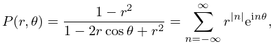
Poisson Kernel
| 1.15.12 | |||
| , | |||
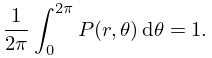
| 1.15.13 | |||
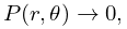
As
| 1.15.14 | |||
uniformly for . (Here and elsewhere in this subsection is a constant such that .)
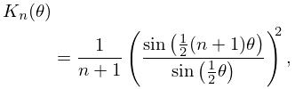
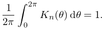
Fejér Kernel
For ,
| 1.15.15 | |||
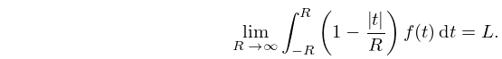
| 1.15.16 | |||
As
| 1.15.17 | |||
uniformly for .
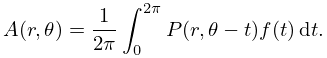
Abel Means
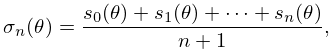
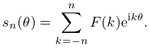
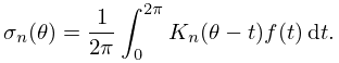
Cesàro (or (C,1)) Means
Let
| 1.15.21 | |||
, where
| 1.15.22 | |||
Then
| 1.15.23 | |||
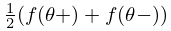
Convergence
If is periodic and integrable on , then as the Abel means and the (C,1) means converge to
| 1.15.24 | |||
at every point where both limits exist. If is also continuous, then the convergence is uniform for all .
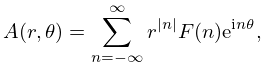
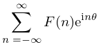
For real-valued , if
| 1.15.25 | |||
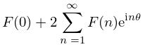
is the Fourier series of , then the series
| 1.15.26 | |||
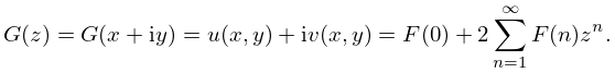
can be extended to the interior of the unit circle as an analytic function
| 1.15.27 | |||
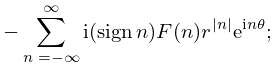
Here is the Abel (or Poisson) sum of , and has the series representation
| 1.15.28 | |||
compare §1.15(v).
§1.15(iv) Definitions for Integrals
Abel Summability
is Abel summable to , or
| 1.15.29 | |||
when
| 1.15.30 | |||
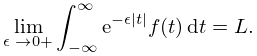
Cesàro Summability
is (C,1) summable to , or
| 1.15.31 | |||
when
| 1.15.32 | |||
If converges and equals , then the integral is Abel and Cesàro summable to .
§1.15(v) Summability of Fourier Integrals
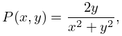
Poisson Kernel
| 1.15.33 | |||
| , . | |||
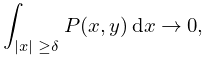
| 1.15.34 | |||
For each ,
| 1.15.35 | |||
| as . | |||
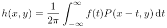
Let
| 1.15.36 | |||
where is the Fourier transform of (§1.14(i)). Then
| 1.15.37 | |||
is the Poisson integral of .
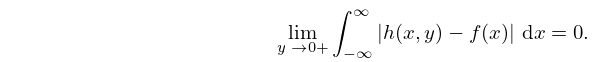
If is integrable on , then
| 1.15.38 | |||
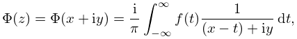
Suppose now is real-valued and integrable on . Let
| 1.15.39 | |||
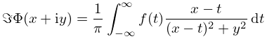
where and . Then is an analytic function in the upper half-plane and its real part is the Poisson integral ; compare (1.9.34). The imaginary part
| 1.15.40 | |||
is the conjugate Poisson integral of . Moreover, is the Hilbert transform of (§1.14(v)).
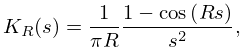
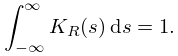
Fejér Kernel
| 1.15.41 | |||
| 1.15.42 | |||
For each ,
| 1.15.43 | |||
| as . | |||
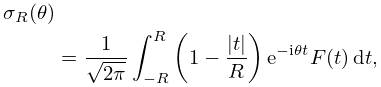
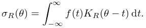
Let
| 1.15.44 | ||||
| then | ||||
| 1.15.45 | ||||
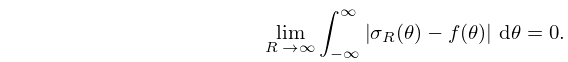
If is integrable on , then
| 1.15.46 | |||
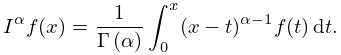
§1.15(vi) Fractional Integrals
For and , the Riemann-Liouville fractional integral of order is defined by
| 1.15.47 | |||
For see §5.2, and compare (1.4.31) in the case when is a positive integer.
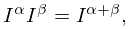
| 1.15.48 | |||
| , . | |||
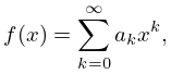
If
| 1.15.49 | |||
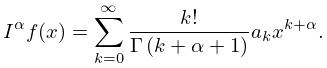
then
| 1.15.50 | |||
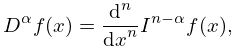
§1.15(vii) Fractional Derivatives
For , an integer, and , the fractional derivative of order is defined by
| 1.15.51 | |||
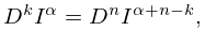
and satisfies the property
| 1.15.52 | |||
| . | |||
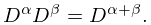
When none of , , and is an integer
| 1.15.53 | |||
Note that . See also Love (1972b).
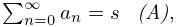
§1.15(viii) Tauberian Theorems
If
| 1.15.54 | ||||
| , | ||||
| , , | ||||
then
| 1.15.55 | |||
If
| 1.15.56 | |||
and either or , then
| 1.15.57 | |||
