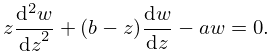
About the Project

Kummer equation

AdvancedHelp

(0.003 seconds)

1—10 of 39 matching pages

1: 13.2 Definitions and Basic Properties
β–Ί
Kummer’s Equation
β–Ί
13.2.1 z ⁒ d 2 w d z 2 + ( b z ) ⁒ d w d z a ⁒ w = 0 .
β–Ί
Standard Solutions
β–Ί
§13.2(v) Numerically Satisfactory Solutions
β–Ί
2: 13.3 Recurrence Relations and Derivatives
β–ΊKummer’s differential equation (13.2.1) is equivalent to … β–Ί
13.3.14 ( a + 1 ) ⁒ z ⁒ U ⁑ ( a + 2 , b + 2 , z ) + ( z b ) ⁒ U ⁑ ( a + 1 , b + 1 , z ) U ⁑ ( a , b , z ) = 0 .
3: 13.14 Definitions and Basic Properties
β–Ί
Whittaker’s Equation
β–ΊThis equation is obtained from Kummer’s equation (13.2.1) via the substitutions W = e 1 2 ⁒ z ⁒ z 1 2 + ΞΌ ⁒ w , ΞΊ = 1 2 ⁒ b a , and ΞΌ = 1 2 ⁒ b 1 2 . … β–ΊStandard solutions are: … β–ΊThe principal branches correspond to the principal branches of the functions z 1 2 + ΞΌ and U ⁑ ( 1 2 + ΞΌ ΞΊ , 1 + 2 ⁒ ΞΌ , z ) on the right-hand sides of the equations (13.14.2) and (13.14.3); compare §4.2(i). …
4: 15.10 Hypergeometric Differential Equation
β–Ί
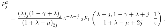
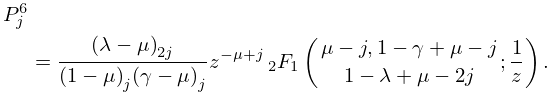
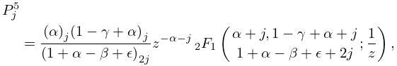
§15.10(ii) Kummer’s 24 Solutions and Connection Formulas
5: 13.29 Methods of Computation
β–Ί
§13.29(ii) Differential Equations
β–ΊA comprehensive and powerful approach is to integrate the differential equations (13.2.1) and (13.14.1) by direct numerical methods. … β–ΊThe integral representations (13.4.1) and (13.4.4) can be used to compute the Kummer functions, and (13.16.1) and (13.16.5) for the Whittaker functions. In Allasia and Besenghi (1991) and Allasia and Besenghi (1987a) the high accuracy of the trapezoidal rule for the computation of Kummer functions is described. … β–ΊIn Colman et al. (2011) an algorithm is described that uses expansions in continued fractions for high-precision computation of M ⁑ ( n , b , x ) , when b and x are real and n is a positive integer. …
6: Errata
β–Ί
  • Equations (13.2.9), (13.2.10)

    There were clarifications made in the conditions on the parameter a in U ⁑ ( a , b , z ) of those equations.

  • β–Ί
  • Subsection 13.8(iii)

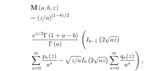
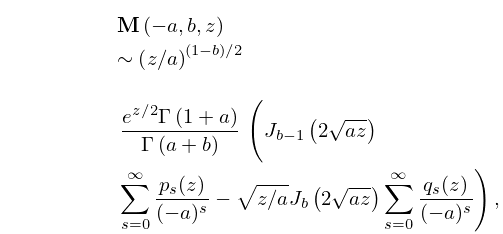
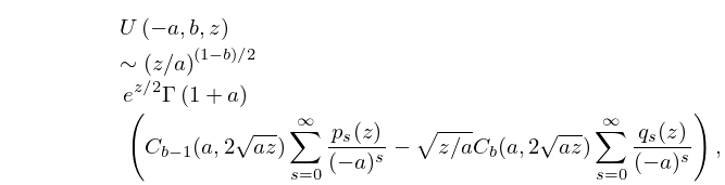
    A new paragraph with several new equations and a new reference has been added at the end to provide asymptotic expansions for Kummer functions U ⁑ ( a , b , z ) and 𝐌 ⁑ ( a , b , z ) as a in | ph ⁑ a | Ο€ Ξ΄ and b and z fixed.

  • β–Ί
  • Equation (13.2.7)
    13.2.7 U ⁑ ( m , b , z ) = ( 1 ) m ⁒ ( b ) m ⁒ M ⁑ ( m , b , z ) = ( 1 ) m ⁒ s = 0 m ( m s ) ⁒ ( b + s ) m s ⁒ ( z ) s

    The equality U ⁑ ( m , b , z ) = ( 1 ) m ⁒ ( b ) m ⁒ M ⁑ ( m , b , z ) has been added to the original equation to express an explicit connection between the two standard solutions of Kummer’s equation. Note also that the notation a = n has been changed to a = m .

    Reported 2015-02-10 by Adri Olde Daalhuis.

  • β–Ί
  • Equation (13.2.8)
    13.2.8 U ⁑ ( a , a + n + 1 , z ) = ( 1 ) n ⁒ ( 1 a n ) n z a + n ⁒ M ⁑ ( n , 1 a n , z ) = z a ⁒ s = 0 n ( n s ) ⁒ ( a ) s ⁒ z s

    The equality U ⁑ ( a , a + n + 1 , z ) = ( 1 ) n ⁒ ( 1 a n ) n z a + n ⁒ M ⁑ ( n , 1 a n , z ) has been added to the original equation to express an explicit connection between the two standard solutions of Kummer’s equation.

    Reported 2015-02-10 by Adri Olde Daalhuis.

  • β–Ί
  • Equation (13.2.10)
    13.2.10 U ⁑ ( m , n + 1 , z ) = ( 1 ) m ⁒ ( n + 1 ) m ⁒ M ⁑ ( m , n + 1 , z ) = ( 1 ) m ⁒ s = 0 m ( m s ) ⁒ ( n + s + 1 ) m s ⁒ ( z ) s

    The equality U ⁑ ( m , n + 1 , z ) = ( 1 ) m ⁒ ( n + 1 ) m ⁒ M ⁑ ( m , n + 1 , z ) has been added to the original equation to express an explicit connection between the two standard solutions of Kummer’s equation. Note also that the notation a = m , m = 0 , 1 , 2 , has been introduced.

    Reported 2015-02-10 by Adri Olde Daalhuis.

  • 7: 31.11 Expansions in Series of Hypergeometric Functions
    β–Ί
    31.11.3_1 P j 5 = ( λ ) j ⁒ ( 1 γ + λ ) j ( 1 + λ μ ) 2 ⁒ j ⁒ z λ j ⁒ F 1 2 ⁑ ( λ + j , 1 γ + λ + j 1 + λ μ + 2 ⁒ j ; 1 z ) ,
    β–Ί
    31.11.3_2 P j 6 = ( λ μ ) 2 ⁒ j ( 1 μ ) j ⁒ ( γ μ ) j ⁒ z μ + j ⁒ F 1 2 ⁑ ( μ j , 1 γ + μ j 1 λ + μ 2 ⁒ j ; 1 z ) .
    β–Ί
    31.11.12 P j 5 = ( α ) j ⁒ ( 1 γ + α ) j ( 1 + α β + ϡ ) 2 ⁒ j ⁒ z α j ⁒ F 1 2 ⁑ ( α + j , 1 γ + α + j 1 + α β + ϡ + 2 ⁒ j ; 1 z ) ,
    8: 13.28 Physical Applications
    §13.28 Physical Applications
    β–Ί
    §13.28(i) Exact Solutions of the Wave Equation
    β–ΊThe reduced wave equation 2 w = k 2 ⁒ w in paraboloidal coordinates, x = 2 ⁒ ΞΎ ⁒ Ξ· ⁒ cos ⁑ Ο• , y = 2 ⁒ ΞΎ ⁒ Ξ· ⁒ sin ⁑ Ο• , z = ΞΎ Ξ· , can be solved via separation of variables w = f 1 ⁑ ( ΞΎ ) ⁒ f 2 ⁑ ( Ξ· ) ⁒ e i ⁒ p ⁒ Ο• , where …and V ΞΊ , ΞΌ ( j ) ⁑ ( z ) , j = 1 , 2 , denotes any pair of solutions of Whittaker’s equation (13.14.1). …
    9: 31.3 Basic Solutions
    β–ΊThe full set of 192 local solutions of (31.2.1), equivalent in 8 sets of 24, resembles Kummer’s set of 24 local solutions of the hypergeometric equation, which are equivalent in 4 sets of 6 solutions (§15.10(ii)); see Maier (2007).
    10: 13.8 Asymptotic Approximations for Large Parameters
    β–Ί
    13.8.11 U ⁑ ( a , b , z ) 2 ⁒ ( z / a ) ( 1 b ) / 2 ⁒ e z / 2 Ξ“ ⁑ ( a ) ⁒ ( K b 1 ⁑ ( 2 ⁒ a ⁒ z ) ⁒ s = 0 p s ⁒ ( z ) a s + z / a ⁒ K b ⁑ ( 2 ⁒ a ⁒ z ) ⁒ s = 0 q s ⁒ ( z ) a s ) ,
    β–Ί
    13.8.12 𝐌 ⁑ ( a , b , z ) ( z / a ) ( 1 b ) / 2 ⁒ e z / 2 ⁒ Ξ“ ⁑ ( 1 + a b ) Ξ“ ⁑ ( a ) ⁒ ( I b 1 ⁑ ( 2 ⁒ a ⁒ z ) ⁒ s = 0 p s ⁒ ( z ) a s z / a ⁒ I b ⁑ ( 2 ⁒ a ⁒ z ) ⁒ s = 0 q s ⁒ ( z ) a s ) ,
    β–Ί
    13.8.13 𝐌 ⁑ ( a , b , z ) ( z / a ) ( 1 b ) / 2 ⁒ e z / 2 ⁒ Ξ“ ⁑ ( 1 + a ) Ξ“ ⁑ ( a + b ) ⁒ ( J b 1 ⁑ ( 2 ⁒ a ⁒ z ) ⁒ s = 0 p s ⁒ ( z ) ( a ) s z / a ⁒ J b ⁑ ( 2 ⁒ a ⁒ z ) ⁒ s = 0 q s ⁒ ( z ) ( a ) s ) ,
    β–Ί
    13.8.14 U ⁑ ( a , b , z ) ( z / a ) ( 1 b ) / 2 ⁒ e z / 2 ⁒ Ξ“ ⁑ ( 1 + a ) ⁒ ( C b 1 ⁒ ( a , 2 ⁒ a ⁒ z ) ⁒ s = 0 p s ⁒ ( z ) ( a ) s z / a ⁒ C b ⁒ ( a , 2 ⁒ a ⁒ z ) ⁒ s = 0 q s ⁒ ( z ) ( a ) s ) ,