Gegenbauer function

SearchAdvancedHelp

(0.002 seconds)

11—20 of 27 matching pages

11: 18.18 Sums

… ►

18.18.8 $$C_n^{(\lambda )}\left(\cos {\theta }_1\cos {\theta }_2+\sin {\theta }_1\sin {\theta }_2\cos \varphi \right)=\sum _{\mathrm{\ell }=0}^n{2}^{2\mathrm{\ell }}(n-\mathrm{\ell })!\frac{2\lambda +2\mathrm{\ell }-1}{2\lambda -1}\frac{{({\left(\lambda \right)}_{\mathrm{\ell }})}^2}{{\left(2\lambda \right)}_{n+\mathrm{\ell }}}{(\sin {\theta }_1)}^{\mathrm{\ell }}{C}_{n-\mathrm{\ell }}^{(\lambda +\mathrm{\ell })}\left(\cos {\theta }_1\right){(\sin {\theta }_2)}^{\mathrm{\ell }}{C}_{n-\mathrm{\ell }}^{(\lambda +\mathrm{\ell })}\left(\cos {\theta }_2\right)C_{\mathrm{\ell }}^{(\lambda -\frac{1}{2})}\left(\cos \varphi \right),$$ $\lambda >0$, $\lambda \ne \frac{1}{2}$.

ⓘ

Symbols:

${\left(a\right)}_n$: Pochhammer’s symbol (or shifted factorial), $\cos z$: cosine function, $!$: factorial (as in $n!$), $\sin z$: sine function, $C_n^{(\lambda )}\left(x\right)$: ultraspherical (or Gegenbauer) polynomial, $\mathrm{\ell }$: nonnegative integer and $n$: nonnegative integer

Referenced by:

§18.17(ii), §18.18(ii), §18.18(ii)

Permalink:

http://dlmf.nist.gov/18.18.E8

Encodings:

pMML, png, TeX

See also:

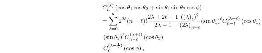
Annotations for §18.18(ii), §18.18(ii), §18.18 and Ch.18

…

12: Bibliography C

… ►

On a generalization of the generating function for Gegenbauer polynomials. Integral Transforms Spec. Funct. 24 (10), pp. 807–816.

ⓘ

External Links:

ISSN 1065-2469, Document, FullText, MathReview Entry, ZentralBlatt

Referenced by:

§14.28(ii), §14.28(ii).

Encodings:

BibTeX

…

13: 10.44 Sums

… ►

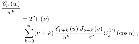
Graf’s and Gegenbauer’s Addition Theorems

…

14: 10.23 Sums

… ►

Graf’s and Gegenbauer’s Addition Theorems

… ►

10.23.8 $$\frac{{𝒞}_{\nu }\left(w\right)}{w^{\nu }}=2^{\nu }\mathrm{\Gamma }\left(\nu \right)\sum _{k=0}^{\mathrm{\infty }}(\nu +k)\frac{{𝒞}_{\nu +k}\left(u\right)}{u^{\nu }}\frac{J_{\nu +k}\left(v\right)}{v^{\nu }}{C}_k^{(\nu )}\left(\cos \alpha \right),$$ $\nu \ne 0,-1,\mathrm{\dots }$, ,

ⓘ

Symbols:

$J_{\nu }\left(z\right)$: Bessel function of the first kind, $\mathrm{\Gamma }\left(z\right)$: gamma function, $\cos z$: cosine function, ${𝒞}_{\nu }\left(z\right)$: cylinder function, $\mathrm{e}$: base of natural logarithm, $\mathrm{i}$: imaginary unit, $C_n^{(\lambda )}\left(x\right)$: ultraspherical (or Gegenbauer) polynomial, $k$: nonnegative integer and $\nu$: complex parameter

A&S Ref:

9.1.80

Referenced by:

§10.23(ii), §10.23(ii), §10.23(ii), §10.44(ii), §10.60(i), §10.60(ii)

Permalink:

http://dlmf.nist.gov/10.23.E8

Encodings:

pMML, png, TeX

See also:

Annotations for §10.23(ii), §10.23(ii), §10.23 and Ch.10

… ►

10.23.9 $${\mathrm{e}}^{\mathrm{i}v\cos \alpha }=\frac{\mathrm{\Gamma }\left(\nu \right)}{{(\frac{1}{2}v)}^{\nu }}\sum _{k=0}^{\mathrm{\infty }}(\nu +k){\mathrm{i}}^k{J}_{\nu +k}\left(v\right)C_k^{(\nu )}\left(\cos \alpha \right),$$ $\nu \ne 0,-1,\mathrm{\dots }$.

ⓘ

Symbols:

$J_{\nu }\left(z\right)$: Bessel function of the first kind, $\mathrm{\Gamma }\left(z\right)$: gamma function, $\cos z$: cosine function, $\mathrm{e}$: base of natural logarithm, $\mathrm{i}$: imaginary unit, $C_n^{(\lambda )}\left(x\right)$: ultraspherical (or Gegenbauer) polynomial, $k$: nonnegative integer and $\nu$: complex parameter

A&S Ref:

9.1.81

Referenced by:

§10.23(ii)

Permalink:

http://dlmf.nist.gov/10.23.E9

Encodings:

pMML, png, TeX

See also:

Annotations for §10.23(ii), §10.23(ii), §10.23 and Ch.10

…

15: 1.10 Functions of a Complex Variable

… ►

§1.10(vi) Multivalued Functions

… ►

§1.10(vii) Inverse Functions

… ►

§1.10(xi) Generating Functions

… ►and hence $\frac{d}{dx}{C}_n^{(\lambda )}\left(x\right)=2\lambda C_{n-1}^{(\lambda +1)}\left(x\right)$, that is (18.9.19). The recurrence relation for $C_n^{(\lambda )}\left(x\right)$ in §18.9(i) follows from $(1-2xz+z^2)\frac{\partial }{\partial z}F(x,\lambda ;z)=2\lambda (x-z)F(x,\lambda ;z)$, and the contour integral representation for $C_n^{(\lambda )}\left(x\right)$ in §18.10(iii) is just (1.10.27).

16: 18.35 Pollaczek Polynomials

… ►

18.35.8 $$P_n^{(\lambda )}(x;0,0)=C_n^{(\lambda )}\left(x\right),$$

ⓘ

Symbols:

$P_n^{(\lambda )}(x;a,b)$: Pollaczek polynomial, $C_n^{(\lambda )}\left(x\right)$: ultraspherical (or Gegenbauer) polynomial, $n$: nonnegative integer and $x$: real variable

Proved:

Ismail (2009, (5.4.3))(proved)

Referenced by:

§18.30(viii), §18.35(i)

Permalink:

http://dlmf.nist.gov/18.35.E8

Encodings:

pMML, png, TeX

See also:

Annotations for §18.35(iii), §18.35 and Ch.18

…

17: 18.3 Definitions

… ►

Table 18.3.1: Orthogonality properties for classical OP’s: intervals, weight functions, standardizations, leading coefficients, and parameter constraints. …

► ►►

Name	$p_n(x)$	$(a,b)$	$w(x)$	$h_n$	$k_n$	${\tilde{k}}_n/k_n$	Constraints
…

►

… ►

18.3.2 $$x_{N+1,n}=\cos \left((n-\frac{1}{2})\pi /(N+1)\right).$$

ⓘ

Symbols:

$\pi$: the ratio of the circumference of a circle to its diameter, $\cos z$: cosine function, $N$: positive integer, $n$: nonnegative integer and $x$: real variable

Permalink:

http://dlmf.nist.gov/18.3.E2

Encodings:

pMML, png, TeX

See also:

Annotations for §18.3, §18.3 and Ch.18

… ►Legendre polynomials are special cases of Legendre functions, Ferrers functions, and associated Legendre functions (§14.7(i)). … ►For $-1-\beta >\alpha >-1$ a finite system of Jacobi polynomials $P_n^{(\alpha ,\beta )}\left(x\right)$ is orthogonal on $(1,\mathrm{\infty })$ with weight function $w(x)={(x-1)}^{\alpha }{(x+1)}^{\beta }$. …

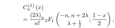
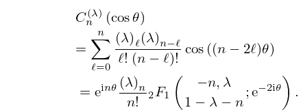
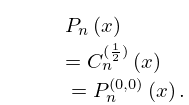
18: 18.5 Explicit Representations

… ►

18.5.9 $$C_n^{(\lambda )}\left(x\right)=\frac{{\left(2\lambda \right)}_n}{n!}{}_2{}^{}F_1^{}(\genfrac{}{}{0pt}{}{-n,n+2\lambda }{\lambda +\frac{1}{2}};\frac{1-x}{2}),$$

ⓘ

Symbols:

${}_2{}^{}F_1^{}(a,b;c;z)$: $=F(a,b;c;z)$ notation for Gauss’ hypergeometric function, ${\left(a\right)}_n$: Pochhammer’s symbol (or shifted factorial), $!$: factorial (as in $n!$), $C_n^{(\lambda )}\left(x\right)$: ultraspherical (or Gegenbauer) polynomial, $n$: nonnegative integer and $x$: real variable

A&S Ref:

22.5.46

Referenced by:

§18.5(iii), §18.6(i)

Permalink:

http://dlmf.nist.gov/18.5.E9

Encodings:

pMML, png, TeX

See also:

Annotations for §18.5(iii), §18.5(iii), §18.5 and Ch.18

►

18.5.10 $$C_n^{(\lambda )}\left(x\right)=\sum _{\mathrm{\ell }=0}^{\lfloor n/2\rfloor }\frac{{(-1)}^{\mathrm{\ell }}{\left(\lambda \right)}_{n-\mathrm{\ell }}}{\mathrm{\ell }!(n-2\mathrm{\ell })!}{(2x)}^{n-2\mathrm{\ell }}={(2x)}^n\frac{{\left(\lambda \right)}_n}{n!}{}_2{}^{}F_1^{}(\genfrac{}{}{0pt}{}{-\frac{1}{2}n,-\frac{1}{2}n+\frac{1}{2}}{1-\lambda -n};\frac{1}{x^2}),$$

ⓘ

Symbols:

${}_2{}^{}F_1^{}(a,b;c;z)$: $=F(a,b;c;z)$ notation for Gauss’ hypergeometric function, ${\left(a\right)}_n$: Pochhammer’s symbol (or shifted factorial), $!$: factorial (as in $n!$), $\lfloor x\rfloor$: floor of $x$ , $C_n^{(\lambda )}\left(x\right)$: ultraspherical (or Gegenbauer) polynomial, $\mathrm{\ell }$: nonnegative integer, $n$: nonnegative integer and $x$: real variable

A&S Ref:

22.3.4

Referenced by:

§18.17(vii), §18.5(iii), §18.6(ii)

Permalink:

http://dlmf.nist.gov/18.5.E10

Encodings:

pMML, png, TeX

See also:

Annotations for §18.5(iii), §18.5(iii), §18.5 and Ch.18

►

18.5.11 $$C_n^{(\lambda )}\left(\cos \theta \right)=\sum _{\mathrm{\ell }=0}^n\frac{{\left(\lambda \right)}_{\mathrm{\ell }}{\left(\lambda \right)}_{n-\mathrm{\ell }}}{\mathrm{\ell }!(n-\mathrm{\ell })!}\cos \left((n-2\mathrm{\ell })\theta \right)={\mathrm{e}}^{\mathrm{i}n\theta }\frac{{\left(\lambda \right)}_n}{n!}{}_2{}^{}F_1^{}(\genfrac{}{}{0pt}{}{-n,\lambda }{1-\lambda -n};{\mathrm{e}}^{-2\mathrm{i}\theta }).$$

ⓘ

Symbols:

${}_2{}^{}F_1^{}(a,b;c;z)$: $=F(a,b;c;z)$ notation for Gauss’ hypergeometric function, ${\left(a\right)}_n$: Pochhammer’s symbol (or shifted factorial), $\cos z$: cosine function, $\mathrm{e}$: base of natural logarithm, $!$: factorial (as in $n!$), $\mathrm{i}$: imaginary unit, $C_n^{(\lambda )}\left(x\right)$: ultraspherical (or Gegenbauer) polynomial, $\mathrm{\ell }$: nonnegative integer and $n$: nonnegative integer

A&S Ref:

22.3.12

Referenced by:

§18.18(iv), §18.5(iii)

Permalink:

http://dlmf.nist.gov/18.5.E11

Encodings:

pMML, png, TeX

See also:

Annotations for §18.5(iii), §18.5(iii), §18.5 and Ch.18

…

19: 18.7 Interrelations and Limit Relations

… ►

18.7.1 $$C_n^{(\lambda )}\left(x\right)=\frac{{\left(2\lambda \right)}_n}{{\left(\lambda +\frac{1}{2}\right)}_n}{P}_n^{(\lambda -\frac{1}{2},\lambda -\frac{1}{2})}\left(x\right),$$

ⓘ

Symbols:

$P_n^{(\alpha ,\beta )}\left(x\right)$: Jacobi polynomial, ${\left(a\right)}_n$: Pochhammer’s symbol (or shifted factorial), $C_n^{(\lambda )}\left(x\right)$: ultraspherical (or Gegenbauer) polynomial, $n$: nonnegative integer and $x$: real variable

A&S Ref:

22.5.27

Referenced by:

§18.15(ii), §18.7(i), §18.7(ii), §18.7(iii)

Permalink:

http://dlmf.nist.gov/18.7.E1

Encodings:

pMML, png, TeX

See also:

Annotations for §18.7(i), §18.7(i), §18.7 and Ch.18

►

18.7.2 $$P_n^{(\alpha ,\alpha )}\left(x\right)=\frac{{\left(\alpha +1\right)}_n}{{\left(2\alpha +1\right)}_n}{C}_n^{(\alpha +\frac{1}{2})}\left(x\right).$$

ⓘ

Symbols:

$P_n^{(\alpha ,\beta )}\left(x\right)$: Jacobi polynomial, ${\left(a\right)}_n$: Pochhammer’s symbol (or shifted factorial), $C_n^{(\lambda )}\left(x\right)$: ultraspherical (or Gegenbauer) polynomial, $n$: nonnegative integer and $x$: real variable

A&S Ref:

22.5.20

Referenced by:

§18.6(i), §18.7(i)

Permalink:

http://dlmf.nist.gov/18.7.E2

Encodings:

pMML, png, TeX

See also:

Annotations for §18.7(i), §18.7(i), §18.7 and Ch.18

►

Chebyshev, Ultraspherical, and Jacobi

… ►

18.7.9 $$P_n\left(x\right)=C_n^{(\frac{1}{2})}\left(x\right)=P_n^{(0,0)}\left(x\right).$$

ⓘ

Symbols:

$P_n^{(\alpha ,\beta )}\left(x\right)$: Jacobi polynomial, $P_n\left(x\right)$: Legendre polynomial, $C_n^{(\lambda )}\left(x\right)$: ultraspherical (or Gegenbauer) polynomial, $n$: nonnegative integer and $x$: real variable

A&S Ref:

22.5.35, 22.5.36

Referenced by:

§10.60(iii), §18.18(ii), §18.5(iii)

Permalink:

http://dlmf.nist.gov/18.7.E9

Encodings:

pMML, png, TeX

See also:

Annotations for §18.7(i), §18.7(i), §18.7 and Ch.18

… ►

18.7.15 $$C_{2n}^{(\lambda )}\left(x\right)=\frac{{\left(\lambda \right)}_n}{{\left(\frac{1}{2}\right)}_n}{P}_n^{(\lambda -\frac{1}{2},-\frac{1}{2})}\left(2x^2-1\right),$$

ⓘ

Symbols:

$P_n^{(\alpha ,\beta )}\left(x\right)$: Jacobi polynomial, ${\left(a\right)}_n$: Pochhammer’s symbol (or shifted factorial), $C_n^{(\lambda )}\left(x\right)$: ultraspherical (or Gegenbauer) polynomial, $n$: nonnegative integer and $x$: real variable

A&S Ref:

22.5.25

Referenced by:

§18.7(ii), §18.9(ii)

Permalink:

http://dlmf.nist.gov/18.7.E15

Encodings:

pMML, png, TeX

See also:

Annotations for §18.7(ii), §18.7 and Ch.18

…

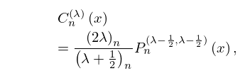
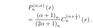
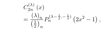
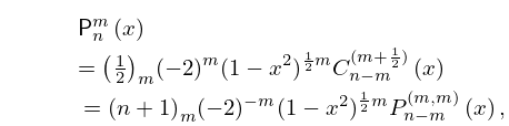
20: 18.11 Relations to Other Functions

… ►

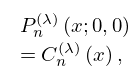
18.11.1 $${𝖯}_n^m\left(x\right)={\left(\frac{1}{2}\right)}_m{(-2)}^m{(1-x^2)}^{\frac{1}{2}m}{C}_{n-m}^{(m+\frac{1}{2})}\left(x\right)={\left(n+1\right)}_m{(-2)}^{-m}{(1-x^2)}^{\frac{1}{2}m}{P}_{n-m}^{(m,m)}\left(x\right),$$ $0\le m\le n$.

ⓘ

Symbols:

: Ferrers function of the first kind, $P_n^{(\alpha ,\beta )}\left(x\right)$: Jacobi polynomial, ${\left(a\right)}_n$: Pochhammer’s symbol (or shifted factorial), $C_n^{(\lambda )}\left(x\right)$: ultraspherical (or Gegenbauer) polynomial, $m$: nonnegative integer, $n$: nonnegative integer and $x$: real variable

Referenced by:

§14.3(iv), §18.11(i)

Permalink:

http://dlmf.nist.gov/18.11.E1

Encodings:

pMML, png, TeX

See also:

Annotations for §18.11(i), §18.11(i), §18.11 and Ch.18

…