18 Orthogonal Polynomials Classical Orthogonal Polynomials 18.2 General Orthogonal Polynomials 18.4 Graphics

§18.3 Definitions

ⓘ

Keywords:: Bochner’s theorem, Chebyshev polynomials, Hermite polynomials, Jacobi polynomials, Laguerre polynomials, Legendre polynomials, Rodrigues formulas, characterizations, classical orthogonal polynomials, degree lowering and raising, differentiation formulas, of coefficients, tables, tables of coefficients, ultraspherical polynomials
Referenced by:: §1.17(iii), §1.17(iii), §1.17(iii), §10.23(ii), §10.54, §10.59, §12.7(i), §13.18(v), §13.6(v), §15.9(i), §15.9(ii), §15.9(iii), §18.2(ii), §18.34(iii), §18.35(iii), §18.38(ii), §28.8(ii), §28.9, §29.15(ii), §29.15(ii), §3.5(v), §3.5(v), §3.5(v), §3.5(v), §3.5(iv), §3.5(v), §31.11(iv), §31.16(ii), §32.10(iv), §34.3(vii), §7.10, §7.18(iv), §7.6(ii), §8.7, Erratum (V1.0.10) for References, Erratum (V1.2.0) Section 18.3
Permalink:: http://dlmf.nist.gov/18.3
Addition (effective with 1.2.0):: Some descriptive text was added under Table 18.3.1.
See also:: Annotations for Ch.18

The classical OP’s comprise the Jacobi, Laguerre and Hermite polynomials. There are many ways of characterizing the classical OP’s within the general OP’s $\{p_{n}(x)\}$ , see Al-Salam (1990). The three most important characterizations are:

1.: As eigenfunctions of second order differential operators (Bochner’s theorem, Bochner (1929)). See the differential equations $A(x)p_{n}^{\prime\prime}(x)+B(x)p_{n}^{\prime}(x)+\lambda_{n}p_{n}(x)=0$ , in Table 18.8.1.
2.: With the property that $\{p_{n+1}^{\prime}(x)\}_{n=0}^{\infty}$ is again a system of OP’s. See §18.9(iii).
3.: As given by a Rodrigues formula (18.5.5).

Table 18.3.1 provides the traditional definitions of Jacobi, Laguerre, and Hermite polynomials via orthogonality and standardization (§§18.2(i) and 18.2(iii)). This table also includes the following special cases of Jacobi polynomials: ultraspherical, Chebyshev, and Legendre.

Table 18.3.1: Orthogonality properties for classical OP’s: intervals, weight functions, standardizations, leading coefficients, and parameter constraints. In the second row

\mathcal{A}_{n}

denotes

\ifrac{2^{\alpha+\beta+1}\Gamma\left(n+\alpha+1\right)\Gamma\left(n+\beta+1% \right)}{((2n+\alpha+\beta+1)\Gamma\left(n+\alpha+\beta+1\right)n!)}

, with

\mathcal{A}_{0}=\ifrac{2^{\alpha+\beta+1}\Gamma\left(\alpha+1\right)\Gamma% \left(\beta+1\right)}{\Gamma\left(\alpha+\beta+2\right)}

. For further implications of the parameter constraints see the Note in §18.5(iii).

Name	$p_{n}(x)$	$(a,b)$	$w(x)$	$h_{n}$	$k_{n}$	$\ifrac{\tilde{k}_{n}}{k_{n}}$	Constraints
Jacobi	$P^{(\alpha,\beta)}_{n}\left(x\right)$	$(-1,1)$	$(1-x)^{\alpha}(1+x)^{\beta}$	$\mathcal{A}_{n}$	$\dfrac{{\left(n+\alpha+\beta+1\right)_{n}}}{2^{n}n!}$	$\dfrac{n(\alpha-\beta)}{2n+\alpha+\beta}$	$\alpha,\beta>-1$
Ultraspherical (Gegenbauer)	$C^{(\lambda)}_{n}\left(x\right)$	$(-1,1)$	$(1-x^{2})^{\lambda-\frac{1}{2}}$	$\dfrac{2^{1-2\lambda}\pi\Gamma\left(n+2\lambda\right)}{(n+\lambda)\left(\Gamma% \left(\lambda\right)\right)^{2}n!}$	$\dfrac{2^{n}{\left(\lambda\right)_{n}}}{n!}$	$0$	$\lambda>-\tfrac{1}{2},\lambda\neq 0$
Chebyshev of first kind	$T_{n}\left(x\right)$	$(-1,1)$	$(1-x^{2})^{-\frac{1}{2}}$	$\begin{cases}\tfrac{1}{2}\pi,&\text{$n>0$}\\ \pi,&\text{$n=0$}\end{cases}$	$\begin{cases}2^{n-1},&\text{$n>0$}\\ 1,&\text{$n=0$}\end{cases}$	$0$
Chebyshev of second kind	$U_{n}\left(x\right)$	$(-1,1)$	$(1-x^{2})^{\frac{1}{2}}$	$\tfrac{1}{2}\pi$	$2^{n}$	$0$
Chebyshev of third kind	$V_{n}\left(x\right)$	$(-1,1)$	$(1-x)^{-\frac{1}{2}}(1+x)^{\frac{1}{2}}$	$\pi$	$2^{n}$	$-\tfrac{1}{2}$
Chebyshev of fourth kind	$W_{n}\left(x\right)$	$(-1,1)$	$(1-x)^{\frac{1}{2}}(1+x)^{-\frac{1}{2}}$	$\pi$	$2^{n}$	$\tfrac{1}{2}$
Shifted Chebyshev of first kind	$T^{*}_{n}\left(x\right)$	$(0,1)$	$(x-x^{2})^{-\frac{1}{2}}$	$\begin{cases}\tfrac{1}{2}\pi,&\text{$n>0$}\\ \pi,&\text{$n=0$}\end{cases}$	$\begin{cases}2^{2n-1},&\text{$n>0$}\\ 1,&\text{$n=0$}\end{cases}$	$-\tfrac{1}{2}n$
Shifted Chebyshev of second kind	$U^{*}_{n}\left(x\right)$	$(0,1)$	$(x-x^{2})^{\frac{1}{2}}$	$\tfrac{1}{8}\pi$	$2^{2n}$	$-\tfrac{1}{2}n$
Legendre	$P_{n}\left(x\right)$	$(-1,1)$	$1$	$\ifrac{2}{(2n+1)}$	$\ifrac{2^{n}{\left(\frac{1}{2}\right)_{n}}}{n!}$	$0$
Shifted Legendre	$P^{*}_{n}\left(x\right)$	$(0,1)$	$1$	$\ifrac{1}{(2n+1)}$	$\ifrac{2^{2n}{\left(\frac{1}{2}\right)_{n}}}{n!}$	$-\frac{1}{2}n$
Laguerre	$L^{(\alpha)}_{n}\left(x\right)$	$(0,\infty)$	${\mathrm{e}}^{-x}x^{\alpha}$	$\ifrac{\Gamma\left(n+\alpha+1\right)}{n!}$	$\ifrac{(-1)^{n}}{n!}$	$-n(n+\alpha)$	$\alpha>-1$
Hermite	$H_{n}\left(x\right)$	$(-\infty,\infty)$	${\mathrm{e}}^{-x^{2}}$	${\pi}^{\frac{1}{2}}2^{n}n!$	$2^{n}$	$0$
Hermite	$\mathit{He}_{n}\left(x\right)$	$(-\infty,\infty)$	${\mathrm{e}}^{-\frac{1}{2}x^{2}}$	$(2\pi)^{\frac{1}{2}}n!$	$1$	$0$

ⓘ

Symbols:: $T_{\NVar{n}}\left(\NVar{x}\right)$ : Chebyshev polynomial of the first kind, $W_{\NVar{n}}\left(\NVar{x}\right)$ : Chebyshev polynomial of the fourth kind, $U_{\NVar{n}}\left(\NVar{x}\right)$ : Chebyshev polynomial of the second kind, $V_{\NVar{n}}\left(\NVar{x}\right)$ : Chebyshev polynomial of the third kind, $\Gamma\left(\NVar{z}\right)$ : gamma function, $H_{\NVar{n}}\left(\NVar{x}\right)$ : Hermite polynomial, $\mathit{He}_{\NVar{n}}\left(\NVar{x}\right)$ : Hermite polynomial, $P^{(\NVar{\alpha},\NVar{\beta})}_{\NVar{n}}\left(\NVar{x}\right)$ : Jacobi polynomial, $L^{(\NVar{\alpha})}_{\NVar{n}}\left(\NVar{x}\right)$ : Laguerre (or generalized Laguerre) polynomial, $P_{\NVar{n}}\left(\NVar{x}\right)$ : Legendre polynomial, ${\left(\NVar{a}\right)_{\NVar{n}}}$ : Pochhammer’s symbol (or shifted factorial), $\pi$ : the ratio of the circumference of a circle to its diameter, $\mathrm{e}$ : base of natural logarithm, $!$ : factorial (as in $n!$ ), $(\NVar{a},\NVar{b})$ : open interval, $T^{*}_{\NVar{n}}\left(\NVar{x}\right)$ : shifted Chebyshev polynomial of the first kind, $U^{*}_{\NVar{n}}\left(\NVar{x}\right)$ : shifted Chebyshev polynomial of the second kind, $P^{*}_{\NVar{n}}\left(\NVar{x}\right)$ : shifted Legendre polynomial, $C^{(\NVar{\lambda})}_{\NVar{n}}\left(\NVar{x}\right)$ : ultraspherical (or Gegenbauer) polynomial, $p_{n}(x)$ : polynomial of degree $n$ , $w(x)$ : weight function, $n$ : nonnegative integer, $x$ : real variable and $h_{n}$
Keywords:: Chebyshev polynomials, Hermite polynomials, Jacobi polynomials, Laguerre polynomials, Legendre polynomials, classical orthogonal polynomials, definition, definitions, leading coefficients, of the first, second, third, and fourth kinds, orthogonality properties, orthogonality property, parameter constraint, parameter constraints, shifted, standardization, standardizations, ultraspherical polynomials, weight function, weight functions, with respect to integration
A&S Ref:: 22.2.1, 22.2.3, 22.2.4, 22.2.5, 22.2.8, 22.2.9, 22.2.10, 22.2.11, 22.2.12, 22.2.13, 22.2.14, 22.2.15, and 22.3.1, 22.3.2, 22.3.4, 22.3.6, 22.3.7, 22.3.8, 22.3.9, 22.3.10, 22.3.11 (see column for $k_{n}$ )
Notes:: In Table 18.3.1, for Row 2 see Szegő (1975, §2.4, Item 1, (4.3.3), and (4.21.6)): the entry in the last column follows from (18.5.7); for Row 3 see Szegő (1975, (4.7.1), (4.7.14), and (4.7.9)): the entry in the last column follows from the symmetry in the fourth row of Table 18.6.1; for Rows 4–7 see Andrews et al. (1999, §5.1 and Remark 2.5.3) and Mason and Handscomb (2003, §4.2.2); for Row 10 specialize Row 2 to $\alpha=\beta=0$ ; for Row 12 see Szegő (1975, §2.4, Item 2, (5.1.1), and (5.1.8)): the entry in the last column follows from (18.5.12); for Row 13 see Szegő (1975, §2.4, Item 3, (5.5.1), and (5.5.6)): the entry in the last column follows from the symmetry in the tenth row of Table 18.6.1.
Referenced by:: §1.18(v), §18.15(vi), (18.17.34_5), §18.2(xi), §18.2(iii), §18.3, Table 18.3.1, §18.3, §18.3, §18.3, §18.30(ii), §18.36(v), §18.39(i), §18.5(i), §18.5(ii), §18.5(iv), §18.7(i), §3.5(v), §3.5(vi), Erratum (V1.0.28) for Table 18.3.1, Erratum (V1.0.28) for Table 18.3.1, Erratum (V1.0.7) for Table 18.3.1, Erratum (V1.0.7) for Table 18.3.1
Permalink:: http://dlmf.nist.gov/18.3.T1
Correction (effective with 1.0.28):: The DLMF now adopts the definitions for the Chebyshev polynomials of the third and fourth kinds $V_{n}\left(x\right)$ , $W_{n}\left(x\right)$ used in Mason and Handscomb (2003). Therefore $V_{n}\left(x\right)$ , $W_{n}\left(x\right)$ , having been interchanged, Rows 5 and 6 have been modified accordingly. For further details see Errata.
Errata (effective with 1.0.7):: The special case of $\mathcal{A}_{n}$ when $n=0$ has been introduced explicitly in the caption for this table. This was needed because the general formula for $\mathcal{A}_{n}$ is undefined at $n=0$ when $\alpha+\beta+1=0$ .
Reported 2013-06-13 by Howard Cohl
See also:: Annotations for §18.3 and Ch.18

For expressions of ultraspherical, Chebyshev, and Legendre polynomials in terms of Jacobi polynomials, see §18.7(i). For representations of the polynomials in Table 18.3.1 by Rodrigues formulas, see §18.5(ii). For finite power series of the Jacobi, ultraspherical, Laguerre, and Hermite polynomials, see §18.5(iii) (in powers of $x-1$ for Jacobi polynomials, in powers of $x$ for the other cases). Explicit power series for Chebyshev, Legendre, Laguerre, and Hermite polynomials for $n=0,1,\ldots,6$ are given in §18.5(iv). For explicit power series coefficients up to $n=12$ for these polynomials and for coefficients up to $n=6$ for Jacobi and ultraspherical polynomials see Abramowitz and Stegun (1964, pp. 793–801).

Chebyshev

ⓘ

Keywords:: Chebyshev polynomials, orthogonality properties, with respect to summation, zeros
Referenced by:: §18.3
Correction (effective with 1.0.28):: The DLMF now adopts the definitions for the Chebyshev polynomials of the third and fourth kinds $V_{n}\left(x\right)$ , $W_{n}\left(x\right)$ , used in Mason and Handscomb (2003), therefore we have interchanged the expressions for $V_{n}\left(x\right)$ , $W_{n}\left(x\right)$ . Since the current definitions are now consistent with Mason and Handscomb (2003), the sentence and reference added in Version Version 1.0.10 (August 7, 2015) has been removed. For further details see Errata.
Addition (effective with 1.0.10):: A sentence and reference to Mason and Handscomb (2003) were added at the end of this paragraph, namely Paragraph Chebyshev.
See also:: Annotations for §18.3 and Ch.18

In this chapter, formulas for the Chebyshev polynomials of the second, third, and fourth kinds will not be given as extensively as those of the first kind. However, most of these formulas can be obtained by specialization of formulas for Jacobi polynomials, via (18.7.4)–(18.7.6).

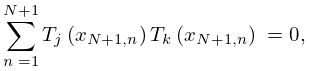
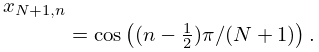
In addition to the orthogonal property given by Table 18.3.1, the Chebyshev polynomials $T_{n}\left(x\right)$ , $n=0,1,\dots,N$ , are orthogonal on the discrete point set comprising the zeros $x_{N+1,n},n=1,2,\dots,N+1$ , of $T_{N+1}\left(x\right)$ :

18.3.1		${\sum_{n=1}^{N+1}T_{j}\left(x_{N+1,n}\right)T_{k}\left(x_{N+1,n}\right)=0},$
$0\leq j\leq N$ , $0\leq k\leq N$ , $j\neq k$ ,
ⓘ Symbols: $T_{\NVar{n}}\left(\NVar{x}\right)$ : Chebyshev polynomial of the first kind, $N$ : positive integer, $n$ : nonnegative integer and $x$ : real variable Referenced by: §18.3, §18.3 Permalink: http://dlmf.nist.gov/18.3.E1 Encodings: TeX, pMML, png See also: Annotations for §18.3, §18.3 and Ch.18

where

18.3.2		$x_{N+1,n}=\cos\left((n-\tfrac{1}{2})\pi/(N+1)\right).$
ⓘ Symbols: $\pi$ : the ratio of the circumference of a circle to its diameter, $\cos\NVar{z}$ : cosine function, $N$ : positive integer, $n$ : nonnegative integer and $x$ : real variable Permalink: http://dlmf.nist.gov/18.3.E2 Encodings: TeX, pMML, png See also: Annotations for §18.3, §18.3 and Ch.18

When $j=k\neq 0$ the sum in (18.3.1) is $\tfrac{1}{2}(N+1)$ . When $j=k=0$ the sum in (18.3.1) is $N+1$ .

For proofs of these results and for similar properties of the Chebyshev polynomials of the second, third, and fourth kinds see Mason and Handscomb (2003, §4.6).

For another version of the discrete orthogonality property of the polynomials $T_{n}\left(x\right)$ see (3.11.9).

Formula (18.3.1) can be understood as a Gauss-Chebyshev quadrature, see (3.5.22), (3.5.23). It is also related to a discrete Fourier-cosine transform, see Britanak et al. (2007).

Legendre

ⓘ

See also:: Annotations for §18.3 and Ch.18

Legendre polynomials are special cases of Legendre functions, Ferrers functions, and associated Legendre functions (§14.7(i)). In consequence, additional properties are included in Chapter 14.

Jacobi on Other Intervals

ⓘ

See also:: Annotations for §18.3 and Ch.18

For $-1-\beta>\alpha>-1$ a finite system of Jacobi polynomials $P^{(\alpha,\beta)}_{n}\left(x\right)$ is orthogonal on $(1,\infty)$ with weight function $w(x)=(x-1)^{\alpha}(x+1)^{\beta}$ . For $\nu\in\mathbb{R}$ and $N>-\tfrac{1}{2}$ a finite system of Jacobi polynomials $P^{(-N-1+\mathrm{i}\nu,-N-1-\mathrm{i}\nu)}_{n}\left(\mathrm{i}x\right)$ (called pseudo Jacobi polynomials or Routh–Romanovski polynomials) is orthogonal on $(-\infty,\infty)$ with $w(x)=\left(1+x^{2}\right)^{-N-1}{\mathrm{e}}^{2\nu\operatorname{arctan}x}$ . For further details see Koekoek et al. (2010, (9.8.3) and §9.9).

Bessel polynomials

ⓘ

See also:: Annotations for §18.3 and Ch.18

Bessel polynomials are often included among the classical OP’s. However, in general they are not orthogonal with respect to a positive measure, but a finite system has such an orthogonality. See §18.34.

18.2 General Orthogonal Polynomials 18.4 Graphics

Site Privacy Accessibility Privacy Program Copyrights Vulnerability Disclosure No Fear Act Policy FOIA Environmental Policy Scientific Integrity Information Quality Standards Commerce.gov Science.gov USA.gov