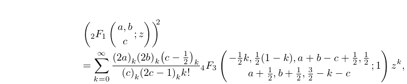
About the Project

Gauss 2F1(-1) sum

AdvancedHelp

(0.015 seconds)

11—20 of 818 matching pages

11: 3.5 Quadrature
§3.5(v) Gauss Quadrature
Gauss–Legendre Formula
Gauss–Chebyshev Formula
Gauss–Jacobi Formula
Gauss–Laguerre Formula
12: 4.38 Inverse Hyperbolic Functions: Further Properties
4.38.5 arctanh z = z + z 3 3 + z 5 5 + z 7 7 + , | z | 1 , z ± 1 .
4.38.15 Arcsinh u ± Arcsinh v = Arcsinh ( u ( 1 + v 2 ) 1 / 2 ± v ( 1 + u 2 ) 1 / 2 ) ,
4.38.17 Arctanh u ± Arctanh v = Arctanh ( u ± v 1 ± u v ) ,
4.38.18 Arcsinh u ± Arccosh v = Arcsinh ( u v ± ( ( 1 + u 2 ) ( v 2 1 ) ) 1 / 2 ) = Arccosh ( v ( 1 + u 2 ) 1 / 2 ± u ( v 2 1 ) 1 / 2 ) ,
4.38.19 Arctanh u ± Arccoth v = Arctanh ( u v ± 1 v ± u ) = Arccoth ( v ± u u v ± 1 ) .
13: 4.13 Lambert W -Function
The decreasing solution can be identified as W ± 1 ( x 0 i ) . …where ln k ( z ) = ln ( z ) + 2 π i k . W 0 ( z ) is a single-valued analytic function on ( , e 1 ] , real-valued when z > e 1 , and has a square root branch point at z = e 1 . …The other branches W k ( z ) are single-valued analytic functions on ( , 0 ] , have a logarithmic branch point at z = 0 , and, in the case k = ± 1 , have a square root branch point at z = e 1 0 i respectively. … where t 0 for W 0 , t 0 for W ± 1 on the relevant branch cuts, …
14: 16.12 Products
16.12.3 ( F 1 2 ( a , b c ; z ) ) 2 = k = 0 ( 2 a ) k ( 2 b ) k ( c 1 2 ) k ( c ) k ( 2 c 1 ) k k ! F 3 4 ( 1 2 k , 1 2 ( 1 k ) , a + b c + 1 2 , 1 2 a + 1 2 , b + 1 2 , 3 2 k c ; 1 ) z k , | z | < 1 .
15: 33.6 Power-Series Expansions in ρ
where A + 1 = 1 , A + 2 = η / ( + 1 ) , and
33.6.3 ( k + ) ( k 1 ) A k = 2 η A k 1 A k 2 , k = + 3 , + 4 , ,
33.6.4 A k ( η ) = ( i ) k 1 ( k 1 ) ! F 1 2 ( + 1 k , + 1 i η ; 2 + 2 ; 2 ) .
33.6.5 H ± ( η , ρ ) = e ± i θ ( η , ρ ) ( 2 + 1 ) ! Γ ( ± i η ) ( k = 0 ( a ) k ( 2 + 2 ) k k ! ( 2 i ρ ) a + k ( ln ( 2 i ρ ) + ψ ( a + k ) ψ ( 1 + k ) ψ ( 2 + 2 + k ) ) k = 1 2 + 1 ( 2 + 1 ) ! ( k 1 ) ! ( 2 + 1 k ) ! ( 1 a ) k ( 2 i ρ ) a k ) ,
where a = 1 + ± i η and ψ ( x ) = Γ ( x ) / Γ ( x ) 5.2(i)). …
16: 15.3 Graphics
See accompanying text
Figure 15.3.2: F ( 5 , 10 ; 1 ; x ) , 0.023 x 1 . Magnify
See accompanying text
Figure 15.3.3: F ( 1 , 10 ; 10 ; x ) , 3 x 1 . Magnify
See accompanying text
Figure 15.3.4: F ( 5 , 10 ; 1 ; x ) , 1 x 0.022 . Magnify
See accompanying text
Figure 15.3.5: F ( 4 3 , 9 16 ; 14 5 ; x + i y ) , 0 x 2 , 0.5 y 0.5 . … Magnify 3D Help
See accompanying text
Figure 15.3.6: F ( 3 , 3 5 ; u + i v ; 1 2 ) , 6 u 2 , 2 v 2 . … Magnify 3D Help
17: 13.14 Definitions and Basic Properties
It has a regular singularity at the origin with indices 1 2 ± μ , and an irregular singularity at infinity of rank one. … For example, if n = 0 , 1 , 2 , , then … If 2 μ = ± n , where n = 0 , 1 , 2 , , then … In cases when 1 2 κ ± μ = n , where n is a nonnegative integer, … When 2 μ is not an integer …
18: 15.8 Transformations of Variable
Group 2 Group 3
Group 2 Group 1
Group 2 Group 4
Group 4 Group 2
provided that z lies in the intersection of the open disks | z 1 4 ± 1 4 3 i | < 1 2 3 , or equivalently, | ph ( ( 1 z ) / ( 1 + 2 z ) ) | < π / 3 . …
19: 32.8 Rational Solutions
Then for n 2 Then P V  has a rational solution iff one of the following holds with m , n and ε = ± 1 : …
  • (c)

    α = 1 2 a 2 , β = 1 2 ( a + n ) 2 , and γ = m , with m + n even.

  • (d)

    α = 1 2 ( b + n ) 2 , β = 1 2 b 2 , and γ = m , with m + n even.

  • where n , a = ε 1 2 α , b = ε 2 2 β , c = ε 3 2 γ , and d = ε 4 1 2 δ , with ε j = ± 1 , j = 1 , 2 , 3 , 4 , independently, and at least one of a , b , c or d is an integer. …
    20: 19.36 Methods of Computation
    where n = 0 , 1 , 2 , , and … The step from n to n + 1 is an ascending Landen transformation if θ = 1 (leading ultimately to a hyperbolic case of R C ) or a descending Gauss transformation if θ = 1 (leading to a circular case of R C ). … Descending Gauss transformations of Π ( ϕ , α 2 , k ) (see (19.8.20)) are used in Fettis (1965) to compute a large table (see §19.37(iii)). This method loses significant figures in ρ if α 2 and k 2 are nearly equal unless they are given exact values—as they can be for tables. … The function el2 ( x , k c , a , b ) is computed by descending Landen transformations if x is real, or by descending Gauss transformations if x is complex (Bulirsch (1965b)). …