…
►The main functions treated in this chapter are the basic hypergeometric (or
-hypergeometric) function
, the bilateral basic hypergeometric (or bilateral
-hypergeometric) function
, and the
-
analogs of the Appell functions
,
,
, and
.
…
►Fine (1988) uses
for a particular specialization of a
function.
…
►If we denote
and
, then
►
►
►
►
…
…
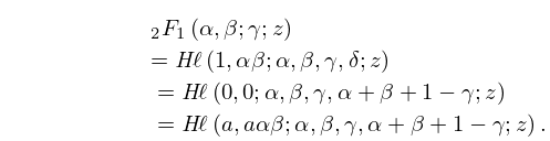
►
31.7.1
►Other reductions of
to a
, with at least one free parameter, exist iff the pair
takes one of a finite number of values, where
.
…
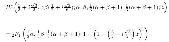
►
31.7.2
►
31.7.3
►
31.7.4
…
…
►
…
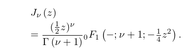
►
10.16.9
►For
see (
16.2.1).
►With
as in §
15.2(i), and with
and
fixed,
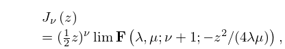
►
10.16.10
…
…
►In no particular order, other generalizations include: Bernoulli numbers and polynomials with arbitrary complex index (
Butzer et al. (1992)); Euler numbers and polynomials with arbitrary complex index (
Butzer et al. (1994));
q-
analogs (
Carlitz (1954a),
Andrews and Foata (1980)); conjugate Bernoulli and Euler polynomials (
Hauss (1997, 1998)); Bernoulli–Hurwitz numbers (
Katz (1975)); poly-Bernoulli numbers (
Kaneko (1997)); Universal Bernoulli numbers (
Clarke (1989));
-adic integer order Bernoulli numbers (
Adelberg (1996));
-adic
-Bernoulli numbers (
Kim and Kim (1999)); periodic Bernoulli numbers (
Berndt (1975b)); cotangent numbers (
Girstmair (1990b)); Bernoulli–Carlitz numbers (
Goss (1978)); Bernoulli–Padé numbers (
Dilcher (2002)); Bernoulli numbers belonging to periodic functions (
Urbanowicz (1988)); cyclotomic Bernoulli numbers (
Girstmair (1990a)); modified Bernoulli numbers (
Zagier (1998)); higher-order Bernoulli and Euler polynomials with multiple parameters (
Erdélyi et al. (1953a, §§1.13.1, 1.14.1)).
…
►
§33.2(ii) Regular Solution
►The function
is recessive (§
2.7(iii)) at
, and is defined by
…
►
§33.2(iii) Irregular Solutions
…
►
and
are complex conjugates, and their real and imaginary parts are given by
…
►As in the case of
, the solutions
and
are analytic functions of
when
.
…
