Buy specialist 60 - www.icmat. - fulfil specialist 40 20mg. ED tables Online - www.icmat.

SearchAdvancedHelp

Did you mean Buy specialist 60 - www.icmat.. - fulfil specialist 40 20mg. ED tables Online - www.icmat.. ?

(0.006 seconds)

1—10 of 248 matching pages

1: Barry I. Schneider

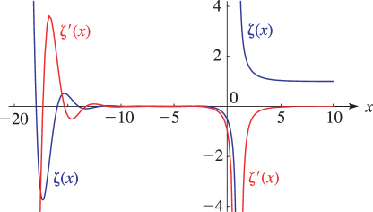
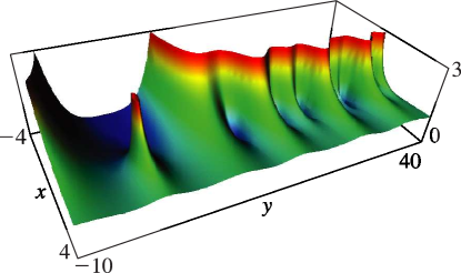
… ►He is an Editor in Chief for Computers in Science and Engineering and a Specialist Editor for Computer Physics Communications. …

2: 25.10 Zeros

… ►More than 41% of all the zeros in the critical strip lie on the critical line (Bui et al. (2011)). …

3: Bibliography B

… ►

Pionic atoms. Annual Review of Nuclear and Particle Science 20, pp. 467–508.

ⓘ

External Links:

Document

Referenced by:

§33.22(iv).

Encodings:

BibTeX

… ►

Coulomb functions (negative energies). Comput. Phys. Comm. 20 (3), pp. 447–458.

ⓘ

Notes:

Double-precision Fortran code.

External Links:

Document, Code

Referenced by:

1st item, 4th item.

Encodings:

BibTeX

… ►

A short table of the functions ${\mathrm{Ki}}_n(x)$, from $n=1$ to $n=16$ . Phil. Mag. Series 7 20, pp. 343–347.

ⓘ

External Links:

Document, ZentralBlatt

Referenced by:

§10.43(iii), 2nd item.

Encodings:

BibTeX

… ►

Occurrence of periodic Lamé functions at bifurcations in chaotic Hamiltonian systems. J. Phys. A 34 (40), pp. 8199–8220.

ⓘ

External Links:

ISSN 0305-4470, Document, MathReview, ZentralBlatt

Referenced by:

§29.19(i).

Encodings:

BibTeX

… ►

More than 41% of the zeros of the zeta function are on the critical line. Acta Arith. 150 (1), pp. 35–64.

ⓘ

External Links:

ISSN 0065-1036, Document, Link, MathReview (Timothy S. Trudgian), ZentralBlatt

Referenced by:

§25.10(ii), §25.10(ii), Erratum (V1.1.4) for Subsection 25.10(ii).

Encodings:

BibTeX

…

4: Errata

… ►

In the paragraph immediately below (25.10.4), it was originally stated that “more than one-third of all zeros in the critical strip lie on the critical line.” which referred to Levinson (1974). This sentence has been updated with “one-third” being replaced with “41%” now referring to Bui et al. (2011) (suggested by Gergő Nemes on 2021-08-23).

… ►

Clarifications were made to this subsection with the addition of Equations (3.5.30_5), (3.5.33_1), (3.5.33_2), (3.5.33_3) and Table 3.5.17_5.

… ►

Special cases of normalization of Jacobi polynomials for which the general formula is undefined have been stated explicitly in Table 18.3.1.

… ►

Several new equations have been added. See (8.17.24), (20.7.34), §20.11(v), (26.12.27), (36.2.28), and (36.2.29).

… ►

Bibliographic citations were added in §§1.13(v), 10.14, 10.21(ii), 18.15(v), 18.32, 30.16(iii), 32.13(ii), and as general references in Chapters 19, 20, 22, and 23.

…

5: 24.20 Tables

§24.20 Tables

… ►Wagstaff (1978) gives complete prime factorizations of $N_n$ and $E_n$ for $n=20(2)60$ and $n=8(2)42$, respectively. In Wagstaff (2002) these results are extended to $n=60(2)152$ and $n=40(2)88$, respectively, with further complete and partial factorizations listed up to $n=300$ and $n=200$, respectively. ►For information on tables published before 1961 see Fletcher et al. (1962, v. 1, §4) and Lebedev and Fedorova (1960, Chapters 11 and 14).

6: 27.2 Functions

… ►Euclid’s Elements (Euclid (1908, Book IX, Proposition 20)) gives an elegant proof that there are infinitely many primes. Tables of primes (§27.21) reveal great irregularity in their distribution. … ►

§27.2(ii) Tables

►Table 27.2.1 lists the first 100 prime numbers $p_n$. Table 27.2.2 tabulates the Euler totient function $\varphi \left(n\right)$, the divisor function $d\left(n\right)$ ($={\sigma }_0(n)$), and the sum of the divisors $\sigma (n)$ ($={\sigma }_1(n)$), for $n=1(1)52$. …

7: 28.35 Tables

… ►

Ince (1932) includes eigenvalues $a_n$, $b_n$, and Fourier coefficients for $n=0$ or $1(1)6$, $q=0(1)10(2)20(4)40$; 7D. Also ${\mathrm{ce}}_n(x,q)$, ${\mathrm{se}}_n(x,q)$ for $q=0(1)10$, $x=1(1)90$, corresponding to the eigenvalues in the tables; 5D. Notation: $a_n={\mathrm{𝑏𝑒}}_n-2q$, $b_n={\mathrm{𝑏𝑜}}_n-2q$.

►

Kirkpatrick (1960) contains tables of the modified functions ${\mathrm{Ce}}_n(x,q)$, ${\mathrm{Se}}_{n+1}(x,q)$ for $n=0(1)5$, $q=1(1)20$, $x=0.1(.1)1$; 4D or 5D.

►

National Bureau of Standards (1967) includes the eigenvalues $a_n\left(q\right)$, $b_n\left(q\right)$ for $n=0(1)3$ with $q=0(.2)20(.5)37(1)100$, and $n=4(1)15$ with $q=0(2)100$; Fourier coefficients for ${\mathrm{ce}}_n(x,q)$ and ${\mathrm{se}}_n(x,q)$ for $n=0(1)15$, $n=1(1)15$, respectively, and various values of $q$ in the interval $[0,100]$; joining factors $g_{e,n}(\sqrt{q})$, $f_{e,n}(\sqrt{q})$ for $n=0(1)15$ with $q=0(.5\text{ to }10)100$ (but in a different notation). Also, eigenvalues for large values of $q$. Precision is generally 8D.

… ►

Zhang and Jin (1996, pp. 521–532) includes the eigenvalues $a_n\left(q\right)$, $b_{n+1}\left(q\right)$ for $n=0(1)4$, $q=0(1)50$; $n=0(1)20$ ($a$’s) or 19 ($b$’s), $q=1,3,5,10,15,25,50(50)200$. Fourier coefficients for ${\mathrm{ce}}_n(x,10)$, ${\mathrm{se}}_{n+1}(x,10)$, $n=0(1)7$. Mathieu functions ${\mathrm{ce}}_n(x,10)$, ${\mathrm{se}}_{n+1}(x,10)$, and their first $x$-derivatives for $n=0(1)4$, $x=0(5^{\circ }){90}^{\circ }$. Modified Mathieu functions ${\mathrm{Mc}}_n^{(j)}(x,\sqrt{10})$, ${\mathrm{Ms}}_{n+1}^{(j)}(x,\sqrt{10})$, and their first $x$-derivatives for $n=0(1)4$, $j=1,2$, $x=0(.2)4$. Precision is mostly 9S.

… ►

Ince (1932) includes the first zero for ${\mathrm{ce}}_n$, ${\mathrm{se}}_n$ for $n=2(1)5$ or $6$, $q=0(1)10(2)40$; 4D. This reference also gives zeros of the first derivatives, together with expansions for small $q$.

…

8: 26.21 Tables

§26.21 Tables

►Abramowitz and Stegun (1964, Chapter 24) tabulates binomial coefficients $\left(\genfrac{}{}{0.0pt}{}{m}{n}\right)$ for $m$ up to 50 and $n$ up to 25; extends Table 26.4.1 to $n=10$; tabulates Stirling numbers of the first and second kinds, $s(n,k)$ and $S(n,k)$, for $n$ up to 25 and $k$ up to $n$; tabulates partitions $p\left(n\right)$ and partitions into distinct parts $p(𝒟,n)$ for $n$ up to 500. ►Andrews (1976) contains tables of the number of unrestricted partitions, partitions into odd parts, partitions into parts $\cancel{\equiv }\pm 2(mod5)$, partitions into parts $\cancel{\equiv }\pm 1(mod5)$, and unrestricted plane partitions up to 100. It also contains a table of Gaussian polynomials up to ${\left[\genfrac{}{}{0.0pt}{}{12}{6}\right]}_q$. ►Goldberg et al. (1976) contains tables of binomial coefficients to $n=100$ and Stirling numbers to $n=40$.

9: 26.2 Basic Definitions

… ►See Table 26.2.1 for $n=0(1)50$. For the actual partitions ($\pi$) for $n=1(1)5$ see Table 26.4.1. … ►

Table 26.2.1: Partitions $p\left(n\right)$.

► ►►►

$n$	$p\left(n\right)$	$n$	$p\left(n\right)$	$n$	$p\left(n\right)$
…
6	11	23	1255	40	37338
…

►

10: 25.3 Graphics

… ►

►►

Figure 25.3.1: Riemann zeta function $\zeta \left(x\right)$ and its derivative ${\zeta }^{\prime }\left(x\right)$, $-20\le x\le 10$. Magnify

… ►

►

►

Figure 25.3.3: Modulus of the Riemann zeta function $|\zeta \left(x+\mathrm{i}y\right)|$, $-4\le x\le 4$, $-10\le y\le 40$. Magnify 3D Help

…