§30.16 Methods of Computation
Contents
- §30.16(i) Eigenvalues
- §30.16(ii) Spheroidal Wave Functions of the First Kind
- §30.16(iii) Radial Spheroidal Wave Functions
§30.16(i) Eigenvalues
For small we can use the power-series expansion (30.3.8). Schäfke and Groh (1962) gives corresponding error bounds. If is large we can use the asymptotic expansions in §30.9. Approximations to eigenvalues can be improved by using the continued-fraction equations from §30.3(iii) and §30.8; see Bouwkamp (1947) and Meixner and Schäfke (1954, §3.93).
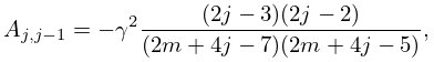
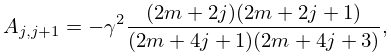
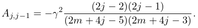
Another method is as follows. Let be even. For sufficiently large, construct the tridiagonal matrix with nonzero elements
| 30.16.1 | ||||
and real eigenvalues , , , , arranged in ascending order of magnitude. Then
| 30.16.2 | |||
and
| 30.16.3 | |||
| . | |||
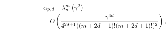
The eigenvalues of can be computed by methods indicated in §§3.2(vi), 3.2(vii). The error satisfies
| 30.16.4 | |||
| . | |||
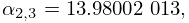
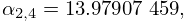
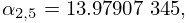
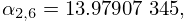
Example
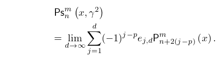
§30.16(ii) Spheroidal Wave Functions of the First Kind
If is large, then we can use the asymptotic expansions referred to in §30.9 to approximate .
If is known, then we can compute (not normalized) by solving the differential equation (30.2.1) numerically with initial conditions , if is even, or , if is odd.
