.6月20足球赛世界杯『wn4.com』国足进过世界杯吗.w6n2c9o.2022年11月29日23时12分3秒.eu6me84ke.cc

SearchAdvancedHelp

(0.005 seconds)

11—20 of 605 matching pages

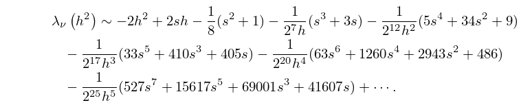
11: 28.16 Asymptotic Expansions for Large $q$

… ►

28.16.1 $${\lambda }_{\nu }\left(h^2\right)\sim -2h^2+2sh-\frac{1}{8}(s^2+1)-\frac{1}{2^{7}h}(s^3+3s)-\frac{1}{2^{12}{h}^2}(5s^4+34s^2+9)-\frac{1}{2^{17}{h}^3}(33s^5+410s^3+405s)-\frac{1}{2^{20}{h}^4}(63s^6+1260s^4+2943s^2+486)-\frac{1}{2^{25}{h}^5}(527s^7+15617s^5+69001s^3+41607s)+\mathrm{\cdots }.$$

ⓘ

Symbols:

${\lambda }_{\nu +2n}\left(q\right)$: eigenvalues of Mathieu equation, $\sim$: Poincaré asymptotic expansion, $h$: parameter and $\nu$: complex parameter

Permalink:

http://dlmf.nist.gov/28.16.E1

Encodings:

pMML, png, TeX

See also:

Annotations for §28.16 and Ch.28

…

12: 8 Incomplete Gamma and Related
Functions

…

13: 28 Mathieu Functions and Hill’s Equation

…

14: 7.24 Approximations

… ►

Cody (1969) provides minimax rational approximations for $\mathrm{erf}x$ and $\mathrm{erfc}x$. The maximum relative precision is about 20S.

… ►

Cody et al. (1970) gives minimax rational approximations to Dawson’s integral $F\left(x\right)$ (maximum relative precision 20S–22S).

… ►

Luke (1969b, pp. 323–324) covers $\frac{1}{2}\sqrt{\pi }\mathrm{erf}x$ and ${\mathrm{e}}^{x^2}F\left(x\right)$ for $-3\le x\le 3$ (the Chebyshev coefficients are given to 20D); $\sqrt{\pi }x{\mathrm{e}}^{x^2}\mathrm{erfc}x$ and $2xF\left(x\right)$ for $x\ge 3$ (the Chebyshev coefficients are given to 20D and 15D, respectively). Coefficients for the Fresnel integrals are given on pp. 328–330 (20D).

►

Bulirsch (1967) provides Chebyshev coefficients for the auxiliary functions $\mathrm{f}\left(x\right)$ and $\mathrm{g}\left(x\right)$ for $x\ge 3$ (15D).

…

15: 23 Weierstrass Elliptic and Modular
Functions

…

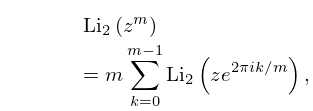
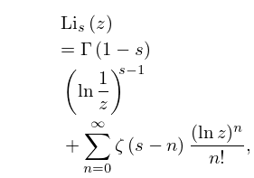
16: 25.12 Polylogarithms

… ►

25.12.5 $${\mathrm{Li}}_2\left(z^m\right)=m\sum _{k=0}^{m-1}{\mathrm{Li}}_2\left(z{\mathrm{e}}^{2\pi \mathrm{i}k/m}\right),$$ $m=1,2,3,\mathrm{\dots }$, .

ⓘ

Symbols:

$\pi$: the ratio of the circumference of a circle to its diameter, ${\mathrm{Li}}_2\left(z\right)$: dilogarithm, $\mathrm{e}$: base of natural logarithm, $\mathrm{i}$: imaginary unit, $k$: nonnegative integer, $m$: nonnegative integer and $z$: complex variable

Source:

Maximon (2003, (3.12), p. 2809)

Permalink:

http://dlmf.nist.gov/25.12.E5

Encodings:

pMML, png, TeX

See also:

Annotations for §25.12(i), §25.12 and Ch.25

… ►

►►

Figure 25.12.1: Dilogarithm function ${\mathrm{Li}}_2\left(x\right)$, Magnify

►

►

►

Figure 25.12.2: Absolute value of the dilogarithm function $\left|{\mathrm{Li}}_2\left(x+\mathrm{i}y\right)\right|$, $-20\le x\le 20$, $-20\le y\le 20$. … Magnify 3D Help

… ►

25.12.12 $${\mathrm{Li}}_s\left(z\right)=\mathrm{\Gamma }\left(1-s\right){\left(\ln \frac{1}{z}\right)}^{s-1}+\sum _{n=0}^{\mathrm{\infty }}\zeta \left(s-n\right)\frac{{(\ln z)}^n}{n!},$$ $s\ne 1,2,3,\mathrm{\dots }$, ,

ⓘ

Symbols:

$\mathrm{\Gamma }\left(z\right)$: gamma function, $\zeta \left(s\right)$: Riemann zeta function, $\pi$: the ratio of the circumference of a circle to its diameter, $!$: factorial (as in $n!$), $\ln z$: principal branch of logarithm function, ${\mathrm{Li}}_s\left(z\right)$: polylogarithm, $n$: nonnegative integer, $s$: complex variable and $z$: complex variable

Keywords:

infinite series, series representation

Source:

Erdélyi et al. (1953a, (1.11.8), p. 29); take $v=1$ and use (25.14.3), (25.11.2)

Permalink:

http://dlmf.nist.gov/25.12.E12

Encodings:

pMML, png, TeX

See also:

Annotations for §25.12(ii), §25.12(ii), §25.12 and Ch.25

…

17: 9.18 Tables

… ►

Miller (1946) tabulates $\mathrm{Ai}\left(x\right)$, ${\mathrm{Ai}}^{\prime }\left(x\right)$ for $x=-20(.01)2;$ ${\log }_{10}\mathrm{Ai}\left(x\right)$, ${\mathrm{Ai}}^{\prime }\left(x\right)/\mathrm{Ai}\left(x\right)$ for $x=0(.1)25(1)75$; $\mathrm{Bi}\left(x\right)$, ${\mathrm{Bi}}^{\prime }\left(x\right)$ for $x=-10(.1)2.5$; ${\log }_{10}\mathrm{Bi}\left(x\right)$, ${\mathrm{Bi}}^{\prime }\left(x\right)/\mathrm{Bi}\left(x\right)$ for $x=0(.1)10$; $M\left(x\right)$, $N\left(x\right)$, $\theta \left(x\right)$, $\varphi \left(x\right)$ (respectively $F(x)$, $G(x)$, $\chi (x)$, $\psi (x)$) for $x=-80(1)-30(.1)0$. Precision is generally 8D; slightly less for some of the auxiliary functions. Extracts from these tables are included in Abramowitz and Stegun (1964, Chapter 10), together with some auxiliary functions for large arguments.

… ►

Zhang and Jin (1996, p. 337) tabulates $\mathrm{Ai}\left(x\right)$, ${\mathrm{Ai}}^{\prime }\left(x\right)$, $\mathrm{Bi}\left(x\right)$, ${\mathrm{Bi}}^{\prime }\left(x\right)$ for $x=0(1)20$ to 8S and for $x=-20(1)0$ to 9D.

… ►

Miller (1946) tabulates $a_k$, ${\mathrm{Ai}}^{\prime }\left(a_k\right)$, $a_k^{\prime }$, $\mathrm{Ai}\left(a_k^{\prime }\right)$, $k=1(1)50$; $b_k$, ${\mathrm{Bi}}^{\prime }\left(b_k\right)$, $b_k^{\prime }$, $\mathrm{Bi}\left(b_k^{\prime }\right)$, $k=1(1)20$. Precision is 8D. Entries for $k=1(1)20$ are reproduced in Abramowitz and Stegun (1964, Chapter 10).

►

Sherry (1959) tabulates $a_k$, ${\mathrm{Ai}}^{\prime }\left(a_k\right)$, $a_k^{\prime }$, $\mathrm{Ai}\left(a_k^{\prime }\right)$, $k=1(1)50$; 20S.

►

Zhang and Jin (1996, p. 339) tabulates $a_k$, ${\mathrm{Ai}}^{\prime }\left(a_k\right)$, $a_k^{\prime }$, $\mathrm{Ai}\left(a_k^{\prime }\right)$, $b_k$, ${\mathrm{Bi}}^{\prime }\left(b_k\right)$, $b_k^{\prime }$, $\mathrm{Bi}\left(b_k^{\prime }\right)$, $k=1(1)20$; 8D.

…

18: 25.20 Approximations

… ►

Cody et al. (1971) gives rational approximations for $\zeta \left(s\right)$ in the form of quotients of polynomials or quotients of Chebyshev series. The ranges covered are $0.5\le s\le 5$, $5\le s\le 11$, $11\le s\le 25$, $25\le s\le 55$. Precision is varied, with a maximum of 20S.

►

Piessens and Branders (1972) gives the coefficients of the Chebyshev-series expansions of $s\zeta \left(s+1\right)$ and $\zeta \left(s+k\right)$, $k=2,3,4,5,8$, for $0\le s\le 1$ (23D).

… ►

Antia (1993) gives minimax rational approximations for $\mathrm{\Gamma }\left(s+1\right)F_s(x)$, where $F_s(x)$ is the Fermi–Dirac integral (25.12.14), for the intervals and , with $s=-\frac{1}{2},\frac{1}{2},\frac{3}{2},\frac{5}{2}$. For each $s$ there are three sets of approximations, with relative maximum errors ${10}^{-4},{10}^{-8},{10}^{-12}$.

19: 28.35 Tables

… ►

Ince (1932) includes eigenvalues $a_n$, $b_n$, and Fourier coefficients for $n=0$ or $1(1)6$, $q=0(1)10(2)20(4)40$; 7D. Also ${\mathrm{ce}}_n(x,q)$, ${\mathrm{se}}_n(x,q)$ for $q=0(1)10$, $x=1(1)90$, corresponding to the eigenvalues in the tables; 5D. Notation: $a_n={\mathrm{𝑏𝑒}}_n-2q$, $b_n={\mathrm{𝑏𝑜}}_n-2q$.

►

Kirkpatrick (1960) contains tables of the modified functions ${\mathrm{Ce}}_n(x,q)$, ${\mathrm{Se}}_{n+1}(x,q)$ for $n=0(1)5$, $q=1(1)20$, $x=0.1(.1)1$; 4D or 5D.

►

National Bureau of Standards (1967) includes the eigenvalues $a_n\left(q\right)$, $b_n\left(q\right)$ for $n=0(1)3$ with $q=0(.2)20(.5)37(1)100$, and $n=4(1)15$ with $q=0(2)100$; Fourier coefficients for ${\mathrm{ce}}_n(x,q)$ and ${\mathrm{se}}_n(x,q)$ for $n=0(1)15$, $n=1(1)15$, respectively, and various values of $q$ in the interval $[0,100]$; joining factors $g_{e,n}(\sqrt{q})$, $f_{e,n}(\sqrt{q})$ for $n=0(1)15$ with $q=0(.5\text{ to }10)100$ (but in a different notation). Also, eigenvalues for large values of $q$. Precision is generally 8D.

… ►

Zhang and Jin (1996, pp. 521–532) includes the eigenvalues $a_n\left(q\right)$, $b_{n+1}\left(q\right)$ for $n=0(1)4$, $q=0(1)50$; $n=0(1)20$ ($a$’s) or 19 ($b$’s), $q=1,3,5,10,15,25,50(50)200$. Fourier coefficients for ${\mathrm{ce}}_n(x,10)$, ${\mathrm{se}}_{n+1}(x,10)$, $n=0(1)7$. Mathieu functions ${\mathrm{ce}}_n(x,10)$, ${\mathrm{se}}_{n+1}(x,10)$, and their first $x$-derivatives for $n=0(1)4$, $x=0(5^{\circ }){90}^{\circ }$. Modified Mathieu functions ${\mathrm{Mc}}_n^{(j)}(x,\sqrt{10})$, ${\mathrm{Ms}}_{n+1}^{(j)}(x,\sqrt{10})$, and their first $x$-derivatives for $n=0(1)4$, $j=1,2$, $x=0(.2)4$. Precision is mostly 9S.

… ►For other tables prior to 1961 see Fletcher et al. (1962, §2.2) and Lebedev and Fedorova (1960, Chapter 11).

20: 36 Integrals with Coalescing Saddles

…