23 Weierstrass Elliptic and Modular Functions Computation 23.21 Physical Applications 23.23 Tables

§23.22 Methods of Computation

Keywords:: Weierstrass elliptic functions
Permalink:: http://dlmf.nist.gov/23.22

§23.22(i) Function Values
§23.22(ii) Lattice Calculations

§23.22(i) Function Values

Keywords:: modular functions
Permalink:: http://dlmf.nist.gov/23.22.i

Given $\omega_{1}$ and $\omega_{3}$ , with $\imagpart{(\omega_{3}/\omega_{1})}>0$ , the nome is computed from $q=e^{{i\pi\omega_{3}/\omega_{1}}}$ . For $\mathop{\wp\/}\nolimits\!\left(z\right)$ we apply (23.6.2) and (23.6.5), generating all needed values of the theta functions by the methods described in §20.14.

The functions $\mathop{\zeta\/}\nolimits\!\left(z\right)$ and $\mathop{\sigma\/}\nolimits\!\left(z\right)$ are computed in a similar manner: the former by replacing and in (23.6.13) by and $\pi z/(2\omega_{1})$ , respectively, and also referring to (23.6.8); the latter by applying (23.6.9).

The modular functions $\mathop{\lambda\/}\nolimits\!\left(\tau\right)$ , $\mathop{J\/}\nolimits\!\left(\tau\right)$ , and $\mathop{\eta\/}\nolimits\!\left(\tau\right)$ are also obtainable in a similar manner from their definitions in §23.15(ii).

§23.22(ii) Lattice Calculations

Notes:: For (23.22.1) combine (23.6.2)–(23.6.4) and §23.10(iv). (23.22.2) and (23.22.3) follow from (23.5.3) and (23.5.7), respectively.
Keywords:: Weierstrass elliptic functions, lattice
Permalink:: http://dlmf.nist.gov/23.22.ii

¶ Starting from Lattice

Suppose that the lattice $\mathbb{L}$ is given. Then a pair of generators $2\omega_{1}$ and $2\omega_{3}$ can be chosen in an almost canonical way as follows. For $2\omega_{1}$ choose a nonzero point of $\mathbb{L}$ of smallest absolute value. (There will be 2, 4, or 6 possible choices.) For $2\omega_{3}$ choose a nonzero point that is not a multiple of $2\omega_{1}$ and is such that $\imagpart{\tau}>0$ and $|\tau|$ is as small as possible, where $\tau=\omega_{3}/\omega_{1}$ . (There will be either 1 or 2 possible choices.) This yields a pair of generators that satisfy $\imagpart{\tau}>0$ , $|\realpart{\tau}|\leq\tfrac{1}{2}$ , $|\tau|>1$ . In consequence, $q=e^{{i\pi\omega_{3}/\omega_{1}}}$ satisfies $|q|\leq e^{{-\pi\sqrt{3}/2}}=0.0658\dots$ . The corresponding values of $e_{1}$ , $e_{2}$ , $e_{3}$ are calculated from (23.6.2)–(23.6.4), then $g_{2}$ and $g_{3}$ are obtained from (23.3.6) and (23.3.7).

¶ Starting from Invariants

Suppose that the invariants $g_{2}=c$ , $g_{3}=d$ , are given, for example in the differential equation (23.3.10) or via coefficients of an elliptic curve (§23.20(ii)). The determination of suitable generators $2\omega_{1}$ and $2\omega_{3}$ is the classical inversion problem (Whittaker and Watson (1927, §21.73), McKean and Moll (1999, §2.12); see also §20.9(i) and McKean and Moll (1999, §2.16)). This problem is solvable as follows:

(a)

In the general case, given by $cd\neq 0$ , we compute the roots $\alpha$ , $\beta$ , $\gamma$ , say, of the cubic equation $4t^{3}-ct-d=0$ ; see §1.11(iii). These roots are necessarily distinct and represent $e_{1}$ , $e_{2}$ , $e_{3}$ in some order.

If and are real, then $e_{1}$ , $e_{2}$ , $e_{3}$ can be identified via (23.5.1), and $k^{2}$ , ${k^{{\prime}}}^{2}$ obtained from (23.6.16).

If and are not both real, then we label $\alpha$ , $\beta$ , $\gamma$ so that the triangle with vertices $\alpha$ , $\beta$ , $\gamma$ is positively oriented and $[\alpha,\gamma]$ is its longest side (chosen arbitrarily if there is more than one). In particular, if $\alpha$ , $\beta$ , $\gamma$ are collinear, then we label them so that $\beta$ is on the line segment $(\alpha,\gamma)$ . In consequence, $k^{2}=(\beta-\gamma)/(\alpha-\gamma)$ , ${k^{{\prime}}}^{2}=(\alpha-\beta)/(\alpha-\gamma)$ satisfy $\imagpart{k^{2}}\geq 0\geq\imagpart{{k^{{\prime}}}^{2}}$ (with strict inequality unless $\alpha$ , $\beta$ , $\gamma$ are collinear); also $|k^{2}|$ , $|{k^{{\prime}}}^{2}|\leq 1$ .

Finally, on taking the principal square roots of $k^{2}$ and ${k^{{\prime}}}^{2}$ we obtain values for and $k^{{\prime}}$ that lie in the 1st and 4th quadrants, respectively, and $2\omega_{1}$ , $2\omega_{3}$ are given by

23.22.1 $2\omega_{1}M(1,k^{{\prime}})=-2i\omega_{3}M(1,k)=\frac{\pi}{3}\sqrt{\frac{c(2+% k^{2}{k^{{\prime}}}^{2})({k^{{\prime}}}^{2}-k^{2})}{d(1-k^{2}{k^{{\prime}}}^{2% })}},$

Symbols:

$\omega_{1}$ , $\omega_{3}$ , $\omega_{2}=-\omega_{1}-\omega_{3}$ : lattice generators, : arithmetic-geometric mean, : modulus and $k^{{\prime}}$ : complementary modulus

Referenced by:

§23.22(ii)

Permalink:

http://dlmf.nist.gov/23.22.E1

Encodings:

TeX, pMML, png

where denotes the arithmetic-geometric mean (see §§19.8(i) and 22.20(ii)). This process yields 2 possible pairs ( $2\omega_{1}$ , $2\omega_{3}$ ), corresponding to the 2 possible choices of the square root.
(b)

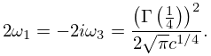
If , then

23.22.2 $2\omega_{1}=-2i\omega_{3}=\frac{\left(\mathop{\Gamma\/}\nolimits\!\left(\frac{% 1}{4}\right)\right)^{2}}{2\sqrt{\pi}c^{{1/4}}}.$

Symbols:

$\mathop{\Gamma\/}\nolimits\!\left(z\right)$ : gamma function and $\omega_{1}$ , $\omega_{3}$ , $\omega_{2}=-\omega_{1}-\omega_{3}$ : lattice generators

Referenced by:

¶ ‣ §22.20(iv), §23.22(ii)

Permalink:

http://dlmf.nist.gov/23.22.E2

Encodings:

TeX, pMML, png

There are 4 possible pairs ( $2\omega_{1}$ , $2\omega_{3}$ ), corresponding to the 4 rotations of a square lattice. The lemniscatic case occurs when and $\omega_{1}>0$ .
(c)

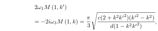
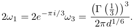
If , then

23.22.3 $2\omega_{1}=2e^{{-\pi i/3}}\omega_{3}=\frac{\left(\mathop{\Gamma\/}\nolimits\!% \left(\frac{1}{3}\right)\right)^{3}}{2\pi d^{{1/6}}}.$

Symbols:

$\mathop{\Gamma\/}\nolimits\!\left(z\right)$ : gamma function, : base of exponential function and $\omega_{1}$ , $\omega_{3}$ , $\omega_{2}=-\omega_{1}-\omega_{3}$ : lattice generators

Referenced by:

§23.22(ii)

Permalink:

http://dlmf.nist.gov/23.22.E3

Encodings:

TeX, pMML, png

There are 6 possible pairs ( $2\omega_{1}$ , $2\omega_{3}$ ), corresponding to the 6 rotations of a lattice of equilateral triangles. The equianharmonic case occurs when and $\omega_{1}>0$ .

¶ Example

Assume $c=g_{2}=-4(3-2i)$ and $d=g_{3}=4(4-2i)$ . Then $\alpha=-1-2i$ , $\beta=1$ , $\gamma=2i$ ; $k^{2}=\ifrac{(7+6i)}{17}$ , and ${k^{{\prime}}}^{2}=\ifrac{(10-6i)}{17}$ . Working to 6 decimal places we obtain