§23.21 Physical Applications
Contents
- §23.21(i) Classical Dynamics
- §23.21(ii) Nonlinear Evolution Equations
- §23.21(iii) Ellipsoidal Coordinates
- §23.21(iv) Modular Functions
§23.21(i) Classical Dynamics
In §22.19(ii) it is noted that Jacobian elliptic functions provide a natural basis of solutions for problems in Newtonian classical dynamics with quartic potentials in canonical form . The Weierstrass function plays a similar role for cubic potentials in canonical form . See, for example, Lawden (1989, Chapter 7) and Whittaker (1964, Chapters 4–6).
§23.21(ii) Nonlinear Evolution Equations
Airault et al. (1977) applies the function to an integrable classical many-body problem, and relates the solutions to nonlinear partial differential equations. For applications to soliton solutions of the Korteweg–de Vries (KdV) equation see McKean and Moll (1999, p. 91), Deconinck and Segur (2000), and Walker (1996, §8.1).
§23.21(iii) Ellipsoidal Coordinates
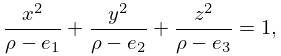
Ellipsoidal coordinates may be defined as the three roots of the equation
| 23.21.1 | |||
where are the corresponding Cartesian coordinates and , , are constants. The Laplacian operator (§1.5(ii)) is given by
| 23.21.2 | |||
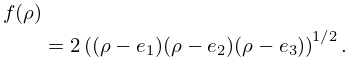
where
| 23.21.3 | |||
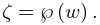
Another form is obtained by identifying , , as lattice roots (§23.3(i)), and setting
| 23.21.4 | ||||
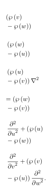
Then
| 23.21.5 | |||
See also §29.18(ii).
