§22.19 Physical Applications
Contents
- §22.19(i) Classical Dynamics: The Pendulum
- §22.19(ii) Classical Dynamics: The Quartic Oscillator
- §22.19(iii) Nonlinear ODEs and PDEs
- §22.19(iv) Tops
- §22.19(v) Other Applications
§22.19(i) Classical Dynamics: The Pendulum
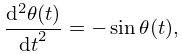
With appropriate scalings, Newton’s equation of motion for a pendulum with a mass in a gravitational field constrained to move in a vertical plane at a fixed distance from a fulcrum is
| 22.19.1 | |||
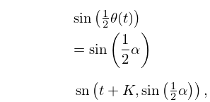
being the angular displacement from the point of stable equilibrium, . The bounded oscillatory solution of (22.19.1) is traditionally written
| 22.19.2 | |||
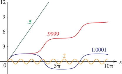
for an initial angular displacement , with at time ; see Lawden (1989, pp. 114–117). The period is . The periodicity and symmetry of the pendulum imply that the motion in each four intervals and have the same “quarter periods” . Thus the offset in 22.19.2 as the motion starts , rather than as in 22.19.3, which follows. The angle is a separatrix, separating oscillatory and unbounded motion. With the same initial conditions, if the sign of gravity is reversed then the new period is ; see Whittaker (1964, §44).
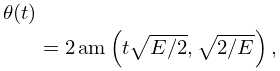
Alternatively, Sala (1989) writes:
| 22.19.3 | |||
for the initial conditions , the point of stable equilibrium for , and . Here is the energy, which is a first integral of the motion. This formulation gives the bounded and unbounded solutions from the same formula (22.19.3), for and , respectively. Also, is not restricted to the principal range . Figure 22.19.1 shows the nature of the solutions of (22.19.3) by graphing for both , as in Figure 22.16.1, and , where it is periodic.
§22.19(ii) Classical Dynamics: The Quartic Oscillator
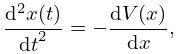
Classical motion in one dimension is described by Newton’s equation
| 22.19.4 | |||
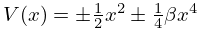
where is the potential energy, and is the coordinate as a function of time . The potential
| 22.19.5 | |||
plays a prototypal role in classical mechanics (Lawden (1989, §5.2)), quantum mechanics (Schulman (1981, Chapter 29)), and quantum field theory (Pokorski (1987, p. 203), Parisi (1988, §14.6)). Its dynamics for purely imaginary time is connected to the theory of instantons (Itzykson and Zuber (1980, p. 572), Schäfer and Shuryak (1998)), to WKB theory, and to large-order perturbation theory (Bender and Wu (1973), Simon (1982)).
For real and positive, three of the four possible combinations of signs give rise to bounded oscillatory motions. We consider the case of a particle of mass 1, initially held at rest at displacement from the origin and then released at time . The subsequent position as a function of time, , for the three cases is given with results expressed in terms of and the dimensionless parameter .
Case I:
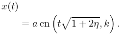
Case II:
There is bounded oscillatory motion near , with period , and modulus , for initial displacements with .
| 22.19.7 | |||
As from below the period diverges since are points of unstable equilibrium.
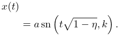
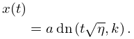
Case III:
Two types of oscillatory motion are possible. For an initial displacement with , bounded oscillations take place near one of the two points of stable equilibrium . Such oscillations, of period , with modulus are given by:
| 22.19.8 | |||
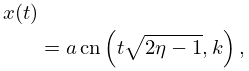
As from below the period diverges since is a point of unstable equlilibrium. For initial displacement with the motion extends over the full range :
| 22.19.9 | |||
with period and modulus . As from above the period again diverges. Both the and solutions approach as from the appropriate directions.
§22.19(iii) Nonlinear ODEs and PDEs
Many nonlinear ordinary and partial differential equations have solutions that may be expressed in terms of Jacobian elliptic functions. These include the time dependent, and time independent, nonlinear Schrödinger equations (NLSE) (Drazin and Johnson (1993, Chapter 2), Ablowitz and Clarkson (1991, pp. 42, 99)), the Korteweg–de Vries (KdV) equation (Kruskal (1974), Li and Olver (2000)), the sine-Gordon equation, and others; see Drazin and Johnson (1993, Chapter 2) for an overview. Such solutions include standing or stationary waves, periodic cnoidal waves, and single and multi-solitons occurring in diverse physical situations such as water waves, optical pulses, quantum fluids, and electrical impulses (Hasegawa (1989), Carr et al. (2000), Kivshar and Luther-Davies (1998), and Boyd (1998, Appendix D2.2)).
§22.19(iv) Tops
The classical rotation of rigid bodies in free space or about a fixed point may be described in terms of elliptic, or hyperelliptic, functions if the motion is integrable (Audin (1999, Chapter 1)). Hyperelliptic functions are solutions of the equation , where is a polynomial of degree higher than 4. Elementary discussions of this topic appear in Lawden (1989, §5.7), Greenhill (1959, pp. 101–103), and Whittaker (1964, Chapter VI). A more abstract overview is Audin (1999, Chapters III and IV), and a complete discussion of analytical solutions in the elliptic and hyperelliptic cases appears in Golubev (1960, Chapters V and VII), the original hyperelliptic investigation being due to Kowalevski (1889).
§22.19(v) Other Applications
Numerous other physical or engineering applications involving Jacobian elliptic functions, and their inverses, to problems of classical dynamics, electrostatics, and hydrodynamics appear in Bowman (1953, Chapters VII and VIII) and Lawden (1989, Chapter 5). Whittaker (1964, Chapter IV) enumerates the complete class of one-body classical mechanical problems that are solvable this way.
