.%E7%94%B7%E7%AF%AE%E4%B8%96%E7%95%8C%E6%9D%AF%E9%A2%84%E9%80%89%E8%B5%9B%E4%B8%AD%E5%9B%BDvs%E9%BB%8E%E5%B7%B4%E5%AB%A9%E3%80%8Ewn4.com%E3%80%8F%E5%92%AA%E5%92%95%E4%B8%96%E7%95%8C%E6%9D%AF%E8%90%A5%E9%94%80%E6%96%B9%E6%A1%88.w6n2c9o.2022%E5%B9%B411%E6%9C%8829%E6%97%A55%E6%97%B652%E5%88%862%E7%A7%92.yeyo8yaka

(0.037 seconds)

11—20 of 666 matching pages

11: Bibliography D

… ►

S. D. Daymond (1955) The principal frequencies of vibrating systems with elliptic boundaries. Quart. J. Mech. Appl. Math. 8 (3), pp. 361–372.

ⓘ

External Links:: Document, MathReview (M. A. Hyman), ZentralBlatt
Referenced by:: 3rd item.
Encodings:: BibTeX

… ►

K. Dilcher (1988) Zeros of Bernoulli, generalized Bernoulli and Euler polynomials. Mem. Amer. Math. Soc. 73 (386), pp. iv+94.

ⓘ

External Links:: ISSN 0065-9266, MathReview (D. H. Lehmer), ZentralBlatt
Referenced by:: §24.12(i), §24.12(iii), §24.16(ii).
Encodings:: BibTeX

… ►

B. Döring (1966) Complex zeros of cylinder functions. Math. Comp. 20 (94), pp. 215–222.

ⓘ

Notes:: For a numerical error in one of the zeros see Amos (1985).
External Links:: ISSN 0025-5718, FullText, MathReview, ZentralBlatt
Referenced by:: 2nd item.
Encodings:: BibTeX

… ►

K. Driver and K. Jordaan (2013) Inequalities for extreme zeros of some classical orthogonal and

q

-orthogonal polynomials. Math. Model. Nat. Phenom. 8 (1), pp. 48–59.

ⓘ

External Links:: ISSN 0973-5348, Document, FullText, MathReview (Ana Foulquié Moreno), ZentralBlatt
Referenced by:: §18.16(ii), §18.16(iv), §18.16(ii), §18.16(iv), §18.27(iv), §18.27(iv), §18.27(v), §18.27(v).
Encodings:: BibTeX

… ►

G. V. Dunne and K. Rao (2000) Lamé instantons. J. High Energy Phys. 2000 (1), pp. Paper 19, 8.

ⓘ

Notes:: (electronic only, article id. JHEP01(2000)019, 8 pp.).
External Links:: ISSN 1029-8479, Document, MathReview, ZentralBlatt
Referenced by:: §22.11.
Encodings:: BibTeX

…

12: Bibliography H

… ►

P. I. Hadži (1972) Certain sums that contain cylindrical functions. Bul. Akad. Štiince RSS Moldoven. 1972 (3), pp. 75–77, 94 (Russian).

ⓘ

External Links:: MathReview (D. P. Gupta)
Referenced by:: §7.14(iii).
Encodings:: BibTeX

… ►

P. I. Hadži (1975a) Certain integrals that contain a probability function. Bul. Akad. Štiince RSS Moldoven. 1975 (2), pp. 86–88, 95 (Russian).

ⓘ

External Links:: MathReview (C. Tanaka)
Referenced by:: §7.14(iii).
Encodings:: BibTeX

… ►

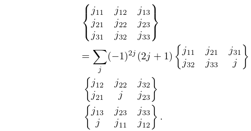
P. I. Hadži (1976a) Expansions for the probability function in series of Čebyšev polynomials and Bessel functions. Bul. Akad. Štiince RSS Moldoven. 1976 (1), pp. 77–80, 96 (Russian).

ⓘ

External Links:: MathReview (V. L. Makarov)
Referenced by:: §7.14(iii).
Encodings:: BibTeX

►

P. I. Hadži (1976b) Integrals that contain a probability function of complicated arguments. Bul. Akad. Štiince RSS Moldoven. 1976 (1), pp. 80–84, 96 (Russian).

ⓘ

External Links:: MathReview (V. L. Makarov)
Referenced by:: §7.14(iii).
Encodings:: BibTeX

►

P. I. Hadži (1978) Sums with cylindrical functions that reduce to the probability function and to related functions. Bul. Akad. Shtiintse RSS Moldoven. 1978 (3), pp. 80–84, 95 (Russian).

ⓘ

External Links:: MathReview (M. Lawrence Glasser)
Referenced by:: §7.14(iii).
Encodings:: BibTeX

…

B. I. Schneider, X. Guan, and K. Bartschat (2016) Time propagation of partial differential equations using the short iterative Lanczos method and finite-element discrete variable representation. Adv. Quantum Chem. 72, pp. 95–127.

ⓘ

Referenced by:: §18.38(i).
Encodings:: BibTeX

… ►

J. B. Seaborn (1991) Hypergeometric Functions and Their Applications. Texts in Applied Mathematics, Vol. 8, Springer-Verlag, New York.

ⓘ

External Links:: ISBN 0-387-97558-6, MathReview (Wolfgang Bühring), ZentralBlatt
Referenced by:: Erratum (V1.2.0) Section 18.39.
Encodings:: BibTeX

… ►

M. J. Seaton (1982) Coulomb functions analytic in the energy. Comput. Phys. Comm. 25 (1), pp. 87–95.

ⓘ

Notes:: Double-precision Fortran code.
External Links:: Document, Code
Referenced by:: §33.1, §33.14(iv), 9th item.
Encodings:: BibTeX

… ►

L. Shen (1981) The elliptical microstrip antenna with circular polarization. IEEE Trans. Antennas and Propagation 29 (1), pp. 90–94.

ⓘ

External Links:: FullText
Referenced by:: 5th item.
Encodings:: BibTeX

… ►

R. Spigler, M. Vianello, and F. Locatelli (1999) Liouville-Green-Olver approximations for complex difference equations. J. Approx. Theory 96 (2), pp. 301–322.

ⓘ

External Links:: ISSN 0021-9045, Document, MathReview (Dumitru Acu), ZentralBlatt
Referenced by:: §2.9(iii).
Encodings:: BibTeX

…

14: Bibliography C

… ►

B. C. Carlson (1977a) Elliptic integrals of the first kind. SIAM J. Math. Anal. 8 (2), pp. 231–242.

ⓘ

External Links:: Document, MathReview (H. E. Fettis), ZentralBlatt
Referenced by:: §19.29(iii).
Encodings:: BibTeX

… ►

B. C. Carlson (1990) Landen Transformations of Integrals. In Asymptotic and Computational Analysis (Winnipeg, MB, 1989), R. Wong (Ed.), Lecture Notes in Pure and Appl. Math., Vol. 124, pp. 75–94.

ⓘ

External Links:: MathReview, ZentralBlatt
Referenced by:: §19.22(iii).
Encodings:: BibTeX

… ►

T. M. Cherry (1948) Expansions in terms of parabolic cylinder functions. Proc. Edinburgh Math. Soc. (2) 8, pp. 50–65.

ⓘ

External Links:: MathReview (I. I. Hirschman, Jr.), ZentralBlatt
Referenced by:: §12.16.
Encodings:: BibTeX

… ►

C. W. Clark (1979) Coulomb phase shift. American Journal of Physics 47 (8), pp. 683–684.

ⓘ

External Links:: Document
Referenced by:: §5.20.
Encodings:: BibTeX

… ►

C. W. Clenshaw, F. W. J. Olver, and P. R. Turner (1989) Level-Index Arithmetic: An Introductory Survey. In Numerical Analysis and Parallel Processing (Lancaster, 1987), P. R. Turner (Ed.), Lecture Notes in Math., Vol. 1397, pp. 95–168.

ⓘ

External Links:: MathReview Entry, ZentralBlatt
Referenced by:: §3.1(iv).
Encodings:: BibTeX

…

15: 23.6 Relations to Other Functions

… ►In this subsection

2\omega_{1}

2\omega_{3}

are any pair of generators of the lattice

\mathbb{L}

, and the lattice roots

e_{1}

e_{2}

e_{3}

are given by (23.3.9). … ►

23.6.2

e_{1}=\frac{\pi^{2}}{12\omega_{1}^{2}}\left({\theta_{2}}^{4}\left(0,q\right)+2% {\theta_{4}}^{4}\left(0,q\right)\right),

ⓘ

Symbols:: $\theta_{\NVar{j}}\left(\NVar{z},\NVar{q}\right)$ : theta function, $e_{\NVar{j}}$ : Weierstrass lattice roots, $\pi$ : the ratio of the circumference of a circle to its diameter, $\mathbb{L}$ : lattice, $q$ : nome and $\omega_{1}$ , $\omega_{3}$ , $\omega_{2}=-\omega_{1}-\omega_{3}$ : lattice generators
A&S Ref:: 18.10.12, 18.10.13, 18.10.14, and 18.10.9, 18.10.10, 18.10.11
Referenced by:: §23.22(ii), §23.22(i), §23.6(i), §23.6(ii)
Permalink:: http://dlmf.nist.gov/23.6.E2
Encodings:: pMML, png, TeX
See also:: Annotations for §23.6(i), §23.6 and Ch.23

… ►Again, in Equations (23.6.16)–(23.6.26),

2\omega_{1},2\omega_{3}

are any pair of generators of the lattice

\mathbb{L}

and

e_{1},e_{2},e_{3}

are given by (23.3.9). … ►Also,

\mathbb{L}_{\mspace{1.0mu}1}

\mathbb{L}_{\mspace{1.0mu}2}

\mathbb{L}_{\mspace{1.0mu}3}

are the lattices with generators

(4K,2\mathrm{i}{K^{\prime}})

(2K-2\mathrm{i}{K^{\prime}},2K+2\mathrm{i}{K^{\prime}})

(2K,4\mathrm{i}{K^{\prime}})

, respectively. … ►Then

z=\wp\left(w\right)

, where the value of

w

depends on the choice of path and determination of the square root; see McKean and Moll (1999, pp. 87–88 and §2.5). …

16: 18.17 Integrals

… ►For the beta function

\mathrm{B}\left(a,b\right)

see §5.12, and for the confluent hypergeometric function

{{}_{1}F_{1}}

see (16.2.1) and Chapter 13. … ►For the confluent hypergeometric function

{{}_{1}F_{1}}

see (16.2.1) and Chapter 13. … ►For the hypergeometric function

{{}_{2}F_{1}}

see §§15.1 and 15.2(i). … ►For the generalized hypergeometric function

{{}_{2}F_{2}}

see (16.2.1). … ►For further integrals, see Apelblat (1983, pp. 189–204), Erdélyi et al. (1954a, pp. 38–39, 94–95, 170–176, 259–261, 324), Erdélyi et al. (1954b, pp. 42–44, 271–294), Gradshteyn and Ryzhik (2000, pp. 788–806), Gröbner and Hofreiter (1950, pp. 23–30), Marichev (1983, pp. 216–247), Oberhettinger (1972, pp. 64–67), Oberhettinger (1974, pp. 83–92), Oberhettinger (1990, pp. 44–47 and 152–154), Oberhettinger and Badii (1973, pp. 103–112), Prudnikov et al. (1986b, pp. 420–617), Prudnikov et al. (1992a, pp. 419–476), and Prudnikov et al. (1992b, pp. 280–308).

17: 34.6 Definition: $\mathit{9j}$ Symbol

§34.6 Definition: $\mathit{9j}$ Symbol

►The

\mathit{9j}

symbol may be defined either in terms of

\mathit{3j}

symbols or equivalently in terms of

\mathit{6j}

symbols: ►

34.6.1

\begin{Bmatrix}j_{11}&j_{12}&j_{13}\\ j_{21}&j_{22}&j_{23}\\ j_{31}&j_{32}&j_{33}\end{Bmatrix}=\sum_{\mbox{\scriptsize all }m_{rs}}\begin{% pmatrix}j_{11}&j_{12}&j_{13}\\ m_{11}&m_{12}&m_{13}\end{pmatrix}\begin{pmatrix}j_{21}&j_{22}&j_{23}\\ m_{21}&m_{22}&m_{23}\end{pmatrix}\begin{pmatrix}j_{31}&j_{32}&j_{33}\\ m_{31}&m_{32}&m_{33}\end{pmatrix}\*\begin{pmatrix}j_{11}&j_{21}&j_{31}\\ m_{11}&m_{21}&m_{31}\end{pmatrix}\begin{pmatrix}j_{12}&j_{22}&j_{32}\\ m_{12}&m_{22}&m_{32}\end{pmatrix}\begin{pmatrix}j_{13}&j_{23}&j_{33}\\ m_{13}&m_{23}&m_{33}\end{pmatrix},

ⓘ

Defines:: $\begin{Bmatrix}\NVar{j_{11}}&\NVar{j_{12}}&\NVar{j_{13}}\\ \NVar{j_{21}}&\NVar{j_{22}}&\NVar{j_{23}}\\ \NVar{j_{31}}&\NVar{j_{32}}&\NVar{j_{33}}\end{Bmatrix}$ : $\mathit{9j}$ symbol
Symbols:: $\begin{pmatrix}\NVar{j_{1}}&\NVar{j_{2}}&\NVar{j_{3}}\\ \NVar{m_{1}}&\NVar{m_{2}}&\NVar{m_{3}}\end{pmatrix}$ : $\mathit{3j}$ symbol, $j,j_{r}$ : non-negative integers or non-negative integers plus one half., $r$ : nonnegative integer and $s$ : integer
Permalink:: http://dlmf.nist.gov/34.6.E1
Encodings:: pMML, png, TeX
See also:: Annotations for §34.6 and Ch.34

►

34.6.2

\begin{Bmatrix}j_{11}&j_{12}&j_{13}\\ j_{21}&j_{22}&j_{23}\\ j_{31}&j_{32}&j_{33}\end{Bmatrix}=\sum_{j}(-1)^{2j}(2j+1)\begin{Bmatrix}j_{11}% &j_{21}&j_{31}\\ j_{32}&j_{33}&j\end{Bmatrix}\begin{Bmatrix}j_{12}&j_{22}&j_{32}\\ j_{21}&j&j_{23}\end{Bmatrix}\begin{Bmatrix}j_{13}&j_{23}&j_{33}\\ j&j_{11}&j_{12}\end{Bmatrix}.

ⓘ

Symbols:: $\begin{Bmatrix}\NVar{j_{11}}&\NVar{j_{12}}&\NVar{j_{13}}\\ \NVar{j_{21}}&\NVar{j_{22}}&\NVar{j_{23}}\\ \NVar{j_{31}}&\NVar{j_{32}}&\NVar{j_{33}}\end{Bmatrix}$ : $\mathit{9j}$ symbol, $\begin{Bmatrix}\NVar{j_{1}}&\NVar{j_{2}}&\NVar{j_{3}}\\ \NVar{l_{1}}&\NVar{l_{2}}&\NVar{l_{3}}\end{Bmatrix}$ : $\mathit{6j}$ symbol and $j,j_{r}$ : non-negative integers or non-negative integers plus one half.
Referenced by:: §34.13
Permalink:: http://dlmf.nist.gov/34.6.E2
Encodings:: pMML, png, TeX
See also:: Annotations for §34.6 and Ch.34

►The

\mathit{9j}

symbol may also be written as a finite triple sum equivalent to a terminating generalized hypergeometric series of three variables with unit arguments. …

18: 19.2 Definitions

… ►The integral for

E\left(\phi,k\right)

is well defined if

k^{2}={\sin}^{2}\phi=1

, and the Cauchy principal value (§1.4(v)) of

\Pi\left(\phi,\alpha^{2},k\right)

is taken if

1-\alpha^{2}{\sin}^{2}\phi

vanishes at an interior point of the integration path. … ►

§19.2(iv) A Related Function: $R_{C}\left(x,y\right)$

… ►Formulas involving

\Pi\left(\phi,\alpha^{2},k\right)

that are customarily different for circular cases, ordinary hyperbolic cases, and (hyperbolic) Cauchy principal values, are united in a single formula by using

R_{C}\left(x,y\right)

. … ►When

x

and

y

are positive,

R_{C}\left(x,y\right)

is an inverse circular function if

x<y

and an inverse hyperbolic function (or logarithm) if

x>y

: …For the special cases of

R_{C}\left(x,x\right)

and

R_{C}\left(0,y\right)

see (19.6.15). …

19: 26.5 Lattice Paths: Catalan Numbers

… ►

C\left(n\right)

is the Catalan number. …(Sixty-six equivalent definitions of

C\left(n\right)

are given in Stanley (1999, pp. 219–229).) … ►

26.5.3

C\left(n+1\right)=\sum_{k=0}^{n}C\left(k\right)C\left(n-k\right),

ⓘ

Symbols:: $C\left(\NVar{n}\right)$ : Catalan number, $k$ : nonnegative integer and $n$ : nonnegative integer
Permalink:: http://dlmf.nist.gov/26.5.E3
Encodings:: pMML, png, TeX
See also:: Annotations for §26.5(iii), §26.5 and Ch.26

►

26.5.4

C\left(n+1\right)=\frac{2(2n+1)}{n+2}C\left(n\right),

ⓘ

Symbols:: $C\left(\NVar{n}\right)$ : Catalan number and $n$ : nonnegative integer
Permalink:: http://dlmf.nist.gov/26.5.E4
Encodings:: pMML, png, TeX
See also:: Annotations for §26.5(iii), §26.5 and Ch.26

… ►

26.5.7

\lim_{n\to\infty}\frac{C\left(n+1\right)}{C\left(n\right)}=4.

ⓘ

Symbols:: $C\left(\NVar{n}\right)$ : Catalan number and $n$ : nonnegative integer
Permalink:: http://dlmf.nist.gov/26.5.E7
Encodings:: pMML, png, TeX
See also:: Annotations for §26.5(iv), §26.5 and Ch.26

20: Bibliography T

… ►

I. C. Tang (1969) Some definite integrals and Fourier series for Jacobian elliptic functions. Z. Angew. Math. Mech. 49, pp. 95–96.

ⓘ

External Links:: ISSN 0044-2267, Document, MathReview (B. C. Carlson), ZentralBlatt
Referenced by:: §22.11.
Encodings:: BibTeX

… ►

N. M. Temme (1994a) A set of algorithms for the incomplete gamma functions. Probab. Engrg. Inform. Sci. 8, pp. 291–307.

ⓘ

Notes:: Includes Pascal program
External Links:: FullText
Referenced by:: §5.24(ii), §7.25(ii), §8.28(ii).
Encodings:: BibTeX

… ►

N. M. Temme (1995b) Bernoulli polynomials old and new: Generalizations and asymptotics. CWI Quarterly 8 (1), pp. 47–66.

ⓘ

External Links:: ISSN 0922-5366, FullText, MathReview (Michael Hauss), ZentralBlatt
Referenced by:: §24.11, §24.16(i).
Encodings:: BibTeX

… ►

P. Terwilliger (2013) The universal Askey-Wilson algebra and DAHA of type

(C^{\vee}_{1},C_{1})

. SIGMA 9, pp. Paper 047, 40 pp..

ⓘ

External Links:: ISSN 1815-0659, Link, MathReview (Renato Álvarez-Nodarse), ZentralBlatt
Referenced by:: §18.38(iii).
Encodings:: BibTeX

… ►

J. Todd (1975) The lemniscate constants. Comm. ACM 18 (1), pp. 14–19.

ⓘ

Notes:: Collection of articles honoring Alston S. Householder. For corrigendum see same journal v. 18 (1975), no. 8, p. 462
External Links:: ISSN 0001-0782, Document, MathReview (L. Fox), ZentralBlatt
Referenced by:: §19.20(i), §19.20(iv), §19.36(iii).
Encodings:: BibTeX

…