matrix exponential

(0.002 seconds)

11—20 of 35 matching pages

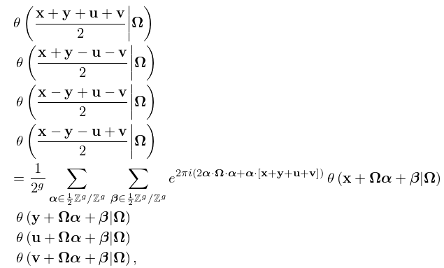
11: 21.5 Modular Transformations

… ►

21.5.4

\theta\left(\left[[\mathbf{C}\boldsymbol{{\Omega}}+\mathbf{D}]^{-1}\right]^{% \mathrm{T}}\mathbf{z}\middle|[\mathbf{A}\boldsymbol{{\Omega}}+\mathbf{B}][% \mathbf{C}\boldsymbol{{\Omega}}+\mathbf{D}]^{-1}\right)=\xi(\boldsymbol{{% \Gamma}})\sqrt{\det[\mathbf{C}\boldsymbol{{\Omega}}+\mathbf{D}]}e^{\pi i% \mathbf{z}\cdot\left[[\mathbf{C}\boldsymbol{{\Omega}}+\mathbf{D}]^{-1}\mathbf{% C}\right]\cdot\mathbf{z}}\theta\left(\mathbf{z}\middle|\boldsymbol{{\Omega}}% \right).

ⓘ

Symbols:: $\theta\left(\NVar{\mathbf{z}}\middle|\NVar{\boldsymbol{{\Omega}}}\right)$ : Riemann theta function, $\pi$ : the ratio of the circumference of a circle to its diameter, $\det$ : determinant, $\mathrm{e}$ : base of natural logarithm, $\mathrm{i}$ : imaginary unit, $\NVar{\mathbf{A}}^{\mathrm{T}}$ : transpose of matrix, $\boldsymbol{{\Omega}}$ : a Riemann matrix, Matrix $\boldsymbol{{\Gamma}}$ and $\xi(\boldsymbol{{\Gamma}})$ : eighth root of unity
Referenced by:: §21.5(i)
Permalink:: http://dlmf.nist.gov/21.5.E4
Encodings:: pMML, png, TeX
See also:: Annotations for §21.5(i), §21.5 and Ch.21

… ►

21.5.9

\theta\genfrac{[}{]}{0.0pt}{}{\mathbf{D}\boldsymbol{{\alpha}}-\mathbf{C}% \boldsymbol{{\beta}}+\tfrac{1}{2}\operatorname{diag}[\mathbf{C}\mathbf{D}^{% \mathrm{T}}]}{-\mathbf{B}\boldsymbol{{\alpha}}+\mathbf{A}\boldsymbol{{\beta}}+% \tfrac{1}{2}\operatorname{diag}[\mathbf{A}\mathbf{B}^{\mathrm{T}}]}\left(\left% [[\mathbf{C}\boldsymbol{{\Omega}}+\mathbf{D}]^{-1}\right]^{\mathrm{T}}\mathbf{% z}\middle|[\mathbf{A}\boldsymbol{{\Omega}}+\mathbf{B}][\mathbf{C}\boldsymbol{{% \Omega}}+\mathbf{D}]^{-1}\right)=\kappa(\boldsymbol{{\alpha}},\boldsymbol{{% \beta}},\boldsymbol{{\Gamma}})\sqrt{\det[\mathbf{C}\boldsymbol{{\Omega}}+% \mathbf{D}]}e^{\pi i\mathbf{z}\cdot\left[[\mathbf{C}\boldsymbol{{\Omega}}+% \mathbf{D}]^{-1}\mathbf{C}\right]\cdot\mathbf{z}}\theta\genfrac{[}{]}{0.0pt}{}% {\boldsymbol{{\alpha}}}{\boldsymbol{{\beta}}}\left(\mathbf{z}\middle|% \boldsymbol{{\Omega}}\right),

ⓘ

Symbols:: $\theta\genfrac{[}{]}{0.0pt}{}{\NVar{\boldsymbol{{\alpha}}}}{\NVar{\boldsymbol{% {\beta}}}}\left(\NVar{\mathbf{z}}\middle|\NVar{\boldsymbol{{\Omega}}}\right)$ : Riemann theta function with characteristics, $\pi$ : the ratio of the circumference of a circle to its diameter, $\det$ : determinant, $\mathrm{e}$ : base of natural logarithm, $\mathrm{i}$ : imaginary unit, $\NVar{\mathbf{A}}^{\mathrm{T}}$ : transpose of matrix, $\boldsymbol{{\Omega}}$ : a Riemann matrix, $\boldsymbol{{\alpha}}$ : $g$ -dimensional vector, $\boldsymbol{{\beta}}$ : $g$ -dimensional vector, $\operatorname{diag}\mathbf{A}$ : Transpose of $[A_{11},A_{22},\ldots,A_{gg}]$ and Matrix $\boldsymbol{{\Gamma}}$
Permalink:: http://dlmf.nist.gov/21.5.E9
Encodings:: pMML, png, TeX
See also:: Annotations for §21.5(ii), §21.5 and Ch.21

…

12: Bibliography D

… ►

P. Deift, T. Kriecherbauer, K. T.-R. McLaughlin, S. Venakides, and X. Zhou (1999b) Uniform asymptotics for polynomials orthogonal with respect to varying exponential weights and applications to universality questions in random matrix theory. Comm. Pure Appl. Math. 52 (11), pp. 1335–1425.

ⓘ

External Links:: ISSN 0010-3640, Document, MathReview (D. S. Lubinsky), ZentralBlatt
Referenced by:: §18.32.
Encodings:: BibTeX

…

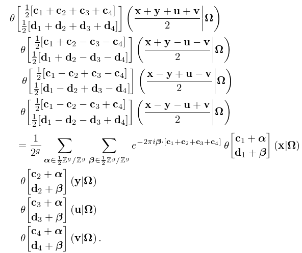
13: 21.6 Products

… ►

21.6.3

\prod_{j=1}^{h}\theta\left(\sum_{k=1}^{h}T_{jk}\mathbf{z}_{k}\middle|% \boldsymbol{{\Omega}}\right)=\frac{1}{\mathcal{D}^{g}}\sum_{\mathbf{A}\in% \mathcal{K}}\sum_{\mathbf{B}\in\mathcal{K}}e^{2\pi i\operatorname{tr}\left[% \frac{1}{2}\mathbf{A}^{\mathrm{T}}\boldsymbol{{\Omega}}\mathbf{A}+\mathbf{A}^{% \mathrm{T}}[\mathbf{Z}+\mathbf{B}]\right]}\*\prod_{j=1}^{h}\theta\left(\mathbf% {z}_{j}+\boldsymbol{{\Omega}}\mathbf{a}_{j}+\mathbf{b}_{j}\middle|\boldsymbol{% {\Omega}}\right),

… ►

21.6.4

\prod_{j=1}^{h}\theta\genfrac{[}{]}{0.0pt}{}{\sum_{k=1}^{h}T_{jk}\mathbf{c}_{k% }}{\sum_{k=1}^{h}T_{jk}\mathbf{d}_{k}}\left(\sum_{k=1}^{h}T_{jk}\mathbf{z}_{k}% \middle|\boldsymbol{{\Omega}}\right)=\frac{1}{\mathcal{D}^{g}}\sum_{\mathbf{A}% \in\mathcal{K}}\sum_{\mathbf{B}\in\mathcal{K}}e^{-2\pi i\sum_{j=1}^{h}\mathbf{% b}_{j}\cdot\mathbf{c}_{j}}\prod_{j=1}^{h}\theta\genfrac{[}{]}{0.0pt}{}{\mathbf% {a}_{j}+\mathbf{c}_{j}}{\mathbf{b}_{j}+\mathbf{d}_{j}}\left(\mathbf{z}_{j}% \middle|\boldsymbol{{\Omega}}\right),

ⓘ

Symbols:: $\theta\genfrac{[}{]}{0.0pt}{}{\NVar{\boldsymbol{{\alpha}}}}{\NVar{\boldsymbol{% {\beta}}}}\left(\NVar{\mathbf{z}}\middle|\NVar{\boldsymbol{{\Omega}}}\right)$ : Riemann theta function with characteristics, $\pi$ : the ratio of the circumference of a circle to its diameter, $\in$ : element of, $\mathrm{e}$ : base of natural logarithm, $\mathrm{i}$ : imaginary unit, $g$ : positive integer, $h$ : positive integer, $\boldsymbol{{\Omega}}$ : a Riemann matrix, $T_{jk}$ : element, $\mathcal{K}$ : set of matrices and $\mathcal{D}$ : number of elements
Permalink:: http://dlmf.nist.gov/21.6.E4
Encodings:: pMML, png, TeX
See also:: Annotations for §21.6(i), §21.6 and Ch.21

… ►

21.6.6

\theta\left(\frac{\mathbf{x}+\mathbf{y}+\mathbf{u}+\mathbf{v}}{2}\middle|% \boldsymbol{{\Omega}}\right)\theta\left(\frac{\mathbf{x}+\mathbf{y}-\mathbf{u}% -\mathbf{v}}{2}\middle|\boldsymbol{{\Omega}}\right)\theta\left(\frac{\mathbf{x% }-\mathbf{y}+\mathbf{u}-\mathbf{v}}{2}\middle|\boldsymbol{{\Omega}}\right)% \theta\left(\frac{\mathbf{x}-\mathbf{y}-\mathbf{u}+\mathbf{v}}{2}\middle|% \boldsymbol{{\Omega}}\right)=\frac{1}{2^{g}}\sum_{\boldsymbol{{\alpha}}\in% \frac{1}{2}{\mathbb{Z}}^{g}/{\mathbb{Z}}^{g}}\,\sum_{\boldsymbol{{\beta}}\in% \frac{1}{2}{\mathbb{Z}}^{g}/{\mathbb{Z}}^{g}}e^{2\pi i\left(2\boldsymbol{{% \alpha}}\cdot\boldsymbol{{\Omega}}\cdot\boldsymbol{{\alpha}}+\boldsymbol{{% \alpha}}\cdot[\mathbf{x}+\mathbf{y}+\mathbf{u}+\mathbf{v}]\right)}\*\theta% \left(\mathbf{x}+\boldsymbol{{\Omega}}\boldsymbol{{\alpha}}+\boldsymbol{{\beta% }}\middle|\boldsymbol{{\Omega}}\right)\theta\left(\mathbf{y}+\boldsymbol{{% \Omega}}\boldsymbol{{\alpha}}+\boldsymbol{{\beta}}\middle|\boldsymbol{{\Omega}% }\right)\theta\left(\mathbf{u}+\boldsymbol{{\Omega}}\boldsymbol{{\alpha}}+% \boldsymbol{{\beta}}\middle|\boldsymbol{{\Omega}}\right)\theta\left(\mathbf{v}% +\boldsymbol{{\Omega}}\boldsymbol{{\alpha}}+\boldsymbol{{\beta}}\middle|% \boldsymbol{{\Omega}}\right),

ⓘ

Symbols:: $\theta\left(\NVar{\mathbf{z}}\middle|\NVar{\boldsymbol{{\Omega}}}\right)$ : Riemann theta function, $\pi$ : the ratio of the circumference of a circle to its diameter, $\in$ : element of, $\mathrm{e}$ : base of natural logarithm, $\mathrm{i}$ : imaginary unit, $\mathbb{Z}$ : set of all integers, $g$ : positive integer, $\boldsymbol{{\Omega}}$ : a Riemann matrix, $\boldsymbol{{\alpha}}$ : $g$ -dimensional vector and $\boldsymbol{{\beta}}$ : $g$ -dimensional vector
Permalink:: http://dlmf.nist.gov/21.6.E6
Encodings:: pMML, png, TeX
See also:: Annotations for §21.6(i), §21.6(i), §21.6 and Ch.21

… ►

21.6.7

\theta\genfrac{[}{]}{0.0pt}{}{\tfrac{1}{2}[\mathbf{c}_{1}+\mathbf{c}_{2}+% \mathbf{c}_{3}+\mathbf{c}_{4}]}{\tfrac{1}{2}[\mathbf{d}_{1}+\mathbf{d}_{2}+% \mathbf{d}_{3}+\mathbf{d}_{4}]}\left(\frac{\mathbf{x}+\mathbf{y}+\mathbf{u}+% \mathbf{v}}{2}\middle|\boldsymbol{{\Omega}}\right)\theta\genfrac{[}{]}{0.0pt}{% }{\tfrac{1}{2}[\mathbf{c}_{1}+\mathbf{c}_{2}-\mathbf{c}_{3}-\mathbf{c}_{4}]}{% \tfrac{1}{2}[\mathbf{d}_{1}+\mathbf{d}_{2}-\mathbf{d}_{3}-\mathbf{d}_{4}]}% \left(\frac{\mathbf{x}+\mathbf{y}-\mathbf{u}-\mathbf{v}}{2}\middle|\boldsymbol% {{\Omega}}\right)\*\theta\genfrac{[}{]}{0.0pt}{}{\tfrac{1}{2}[\mathbf{c}_{1}-% \mathbf{c}_{2}+\mathbf{c}_{3}-\mathbf{c}_{4}]}{\tfrac{1}{2}[\mathbf{d}_{1}-% \mathbf{d}_{2}+\mathbf{d}_{3}-\mathbf{d}_{4}]}\left(\frac{\mathbf{x}-\mathbf{y% }+\mathbf{u}-\mathbf{v}}{2}\middle|\boldsymbol{{\Omega}}\right)\theta\genfrac{% [}{]}{0.0pt}{}{\tfrac{1}{2}[\mathbf{c}_{1}-\mathbf{c}_{2}-\mathbf{c}_{3}+% \mathbf{c}_{4}]}{\tfrac{1}{2}[\mathbf{d}_{1}-\mathbf{d}_{2}-\mathbf{d}_{3}+% \mathbf{d}_{4}]}\left(\frac{\mathbf{x}-\mathbf{y}-\mathbf{u}+\mathbf{v}}{2}% \middle|\boldsymbol{{\Omega}}\right)\\ =\frac{1}{2^{g}}\sum_{\boldsymbol{{\alpha}}\in\frac{1}{2}{\mathbb{Z}}^{g}/{% \mathbb{Z}}^{g}}\,\sum_{\boldsymbol{{\beta}}\in\frac{1}{2}{\mathbb{Z}}^{g}/{% \mathbb{Z}}^{g}}e^{-2\pi i\boldsymbol{{\beta}}\cdot[\mathbf{c}_{1}+\mathbf{c}_% {2}+\mathbf{c}_{3}+\mathbf{c}_{4}]}\*\theta\genfrac{[}{]}{0.0pt}{}{\mathbf{c}_% {1}+\boldsymbol{{\alpha}}}{\mathbf{d}_{1}+\boldsymbol{{\beta}}}\left(\mathbf{x% }\middle|\boldsymbol{{\Omega}}\right)\theta\genfrac{[}{]}{0.0pt}{}{\mathbf{c}_% {2}+\boldsymbol{{\alpha}}}{\mathbf{d}_{2}+\boldsymbol{{\beta}}}\left(\mathbf{y% }\middle|\boldsymbol{{\Omega}}\right)\theta\genfrac{[}{]}{0.0pt}{}{\mathbf{c}_% {3}+\boldsymbol{{\alpha}}}{\mathbf{d}_{3}+\boldsymbol{{\beta}}}\left(\mathbf{u% }\middle|\boldsymbol{{\Omega}}\right)\theta\genfrac{[}{]}{0.0pt}{}{\mathbf{c}_% {4}+\boldsymbol{{\alpha}}}{\mathbf{d}_{4}+\boldsymbol{{\beta}}}\left(\mathbf{v% }\middle|\boldsymbol{{\Omega}}\right).

ⓘ

Symbols:: $\theta\genfrac{[}{]}{0.0pt}{}{\NVar{\boldsymbol{{\alpha}}}}{\NVar{\boldsymbol{% {\beta}}}}\left(\NVar{\mathbf{z}}\middle|\NVar{\boldsymbol{{\Omega}}}\right)$ : Riemann theta function with characteristics, $\pi$ : the ratio of the circumference of a circle to its diameter, $\in$ : element of, $\mathrm{e}$ : base of natural logarithm, $\mathrm{i}$ : imaginary unit, $\mathbb{Z}$ : set of all integers, $g$ : positive integer, $\boldsymbol{{\Omega}}$ : a Riemann matrix, $\boldsymbol{{\alpha}}$ : $g$ -dimensional vector and $\boldsymbol{{\beta}}$ : $g$ -dimensional vector
Permalink:: http://dlmf.nist.gov/21.6.E7
Encodings:: pMML, png, TeX
See also:: Annotations for §21.6(i), §21.6(i), §21.6 and Ch.21

…

14: 28.29 Definitions and Basic Properties

… ►iff

e^{\pi\mathrm{i}\nu}

is an eigenvalue of the matrix …

15: 28.2 Definitions and Basic Properties

… ►iff

e^{\pi\mathrm{i}\nu}

is an eigenvalue of the matrix …

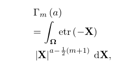
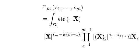
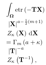
16: 35.3 Multivariate Gamma and Beta Functions

… ►

35.3.1

\Gamma_{m}\left(a\right)=\int_{\boldsymbol{\Omega}}\operatorname{etr}\left(-% \mathbf{X}\right)\left|\mathbf{X}\right|^{a-\frac{1}{2}(m+1)}\,\mathrm{d}{% \mathbf{X}},

\Re\left(a\right)>\frac{1}{2}(m-1)

ⓘ

Symbols:: $\operatorname{etr}\left(\NVar{\mathbf{A}}\right)$ : exponential of trace, $\int$ : integral, $\Gamma_{\NVar{m}}\left(\NVar{a}\right)$ : multivariate gamma function, $\Re$ : real part, $a$ : complex variable, $\mathbf{X}$ : real symmetric $m\times m$ matrix, $\left|\NVar{\mathbf{X}}\right|$ : determinant of $\NVar{\mathbf{X}}$ , $\,\mathrm{d}$ : differential of matrix, ${\boldsymbol{\Omega}}$ : space of positive-definite real symmetric $m\times m$ matrices and $m$ : positive integer
Permalink:: http://dlmf.nist.gov/35.3.E1
Encodings:: pMML, png, TeX
See also:: Annotations for §35.3(i), §35.3 and Ch.35

►

35.3.2

\Gamma_{m}\left(s_{1},\dots,s_{m}\right)=\int_{\boldsymbol{\Omega}}% \operatorname{etr}\left(-\mathbf{X}\right)\left|\mathbf{X}\right|^{s_{m}-\frac% {1}{2}(m+1)}\prod_{j=1}^{m-1}|(\mathbf{X})_{j}|^{s_{j}-s_{j+1}}\,\mathrm{d}{% \mathbf{X}},

s_{j}\in\mathbb{C}

\Re\left(s_{j}\right)>\frac{1}{2}(j-1)

j=1,\dots,m

…

17: 35.4 Partitions and Zonal Polynomials

… ►

35.4.8

\int_{\boldsymbol{\Omega}}\operatorname{etr}\left(-\mathbf{T}\mathbf{X}\right)% \,\left|\mathbf{X}\right|^{a-\frac{1}{2}(m+1)}Z_{\kappa}\left(\mathbf{X}\right% )\,\mathrm{d}{\mathbf{X}}=\Gamma_{m}\left(a+\kappa\right)\,\left|\mathbf{T}% \right|^{-a}Z_{\kappa}\left(\mathbf{T}^{-1}\right),

…

18: 33.22 Particle Scattering and Atomic and Molecular Spectra

… ►With

e

denoting here the elementary charge, the Coulomb potential between two point particles with charges

Z_{1}e,Z_{2}e

and masses

m_{1},m_{2}

separated by a distance

s

V(s)=Z_{1}Z_{2}e^{2}/(4\pi\varepsilon_{0}s)=Z_{1}Z_{2}\alpha\hbar c/s

, where

Z_{j}

are atomic numbers,

\varepsilon_{0}

is the electric constant,

\alpha

is the fine structure constant, and

\hbar

is the reduced Planck’s constant. … ►For

Z_{1}Z_{2}=-1

and

m=m_{e}

, the electron mass, the scaling factors in (33.22.5) reduce to the Bohr radius,

a_{0}=\hbar/(m_{e}c\alpha)

, and to a multiple of the Rydberg constant, ►

R_{\infty}=m_{e}c{\alpha}^{2}/(2\hbar)

. … ►For scattering problems, the interior solution is then matched to a linear combination of a pair of Coulomb functions,

F_{\ell}\left(\eta,\rho\right)

and

G_{\ell}\left(\eta,\rho\right)

, or

f\left(\epsilon,\ell;r\right)

and

h\left(\epsilon,\ell;r\right)

, to determine the scattering

S

-matrix and also the correct normalization of the interior wave solutions; see Bloch et al. (1951). … ►

•

Searches for resonances as poles of the $S$ -matrix in the complex half-plane $\Im\sf{k}<0$ . See for example Csótó and Hale (1997).

…

19: 3.11 Approximation Techniques

… ►The matrix is symmetric and positive definite, but the system is ill-conditioned when

n

is large because the lower rows of the matrix are approximately proportional to one another. … ►Since

X_{k\ell}=X_{\ell k}

, the matrix is again symmetric. … ►We take

n

complex exponentials

\phi_{k}(x)=e^{\mathrm{i}kx}

k=0,1,\dots,n-1

, and approximate

f(x)

by the linear combination (3.11.31). … ►

\omega_{n}=e^{2\pi i/n}

j=0,1,\dots,n-1

… ►The method of the fast Fourier transform (FFT) exploits the structure of the matrix

\boldsymbol{{\Omega}}

with elements

\omega_{n}^{jk}

j,k=0,1,\dots,n-1

. …

20: 32.14 Combinatorics

… ►

32.14.2

F(s)=\exp\left(-\int_{s}^{\infty}(x-s)w^{2}(x)\,\mathrm{d}x\right),

ⓘ

Symbols:: $\,\mathrm{d}\NVar{x}$ : differential of $x$ , $\exp\NVar{z}$ : exponential function, $\int$ : integral, $x$ : real and $F(s)$ : distribution function
Referenced by:: §32.14
Permalink:: http://dlmf.nist.gov/32.14.E2
Encodings:: pMML, png, TeX
See also:: Annotations for §32.14 and Ch.32

… ►The distribution function

F(s)

given by (32.14.2) arises in random matrix theory where it gives the limiting distribution for the normalized largest eigenvalue in the Gaussian Unitary Ensemble of

n\times n

Hermitian matrices; see Tracy and Widom (1994). … ►See Forrester and Witte (2001, 2002) for other instances of Painlevé equations in random matrix theory.