connected point set
(0.003 seconds)
1—10 of 23 matching pages
1: 1.9 Calculus of a Complex Variable
…
►A domain
, say, is an open set in that is connected, that is, any two points can be joined by a polygonal arc (a finite chain of straight-line segments) lying in the set.
…
…
2: 36.5 Stokes Sets
…
►The Stokes set is itself a cusped curve, connected to the cusp of the bifurcation set:
…
►They generate a pair of cusp-edged sheets connected to the cusped sheets of the swallowtail bifurcation set (§36.4).
…
►This consists of a cusp-edged sheet connected to the cusp-edged sheet of the bifurcation set and intersecting the smooth sheet of the bifurcation set.
…
►This part of the Stokes set connects two complex saddles.
…
►In Figure 36.5.4 the part of the Stokes surface inside the bifurcation set connects two complex saddles.
…
3: 23.20 Mathematical Applications
…
►It follows from the addition formula (23.10.1) that the points
, , have zero sum iff , so that addition of points on the curve corresponds to addition of parameters on the torus ; see McKean and Moll (1999, §§2.11, 2.14).
…
►The geometric nature of this construction is illustrated in McKean and Moll (1999, §2.14), Koblitz (1993, §§6, 7), and Silverman and Tate (1992, Chapter 1, §§3, 4): each of these references makes a connection with the addition theorem (23.10.1).
…
►Let denote the set of points on that are of finite order (that is, those points
for which there exists a positive integer with ), and let be the sets of points with integer and rational coordinates, respectively.
…The resulting points are then tested for finite order as follows.
…If any of these quantities is zero, then the point has finite order.
…
4: 1.13 Differential Equations
…
►
§1.13(i) Existence of Solutions
►A domain in the complex plane is simply-connected if it has no “holes”; more precisely, if its complement in the extended plane is connected. … ►where , a simply-connected domain, and , are analytic in , has an infinite number of analytic solutions in . A solution becomes unique, for example, when and are prescribed at a point in . … ►Transformation of the Point at Infinity
…5: 21.7 Riemann Surfaces
…
►
§21.7(i) Connection of Riemann Theta Functions to Riemann Surfaces
… ►Consider the set of points in that satisfy the equation …This compact curve may have singular points, that is, points at which the gradient of vanishes. Removing the singularities of this curve gives rise to a two-dimensional connected manifold with a complex-analytic structure, that is, a Riemann surface. All compact Riemann surfaces can be obtained this way. … ►Denote the set of all branch points by . …6: 7.20 Mathematical Applications
…
►For applications of the complementary error function in uniform asymptotic approximations of integrals—saddle point coalescing with a pole or saddle point coalescing with an endpoint—see Wong (1989, Chapter 7), Olver (1997b, Chapter 9), and van der Waerden (1951).
…
►
§7.20(ii) Cornu’s Spiral
►Let the set be defined by , , . Then the set is called Cornu’s spiral: it is the projection of the corkscrew on the -plane. …Let be any point on the projected spiral. …7: 2.8 Differential Equations with a Parameter
…
►in which is a real or complex parameter, and asymptotic solutions are needed for large that are uniform with respect to in a point set
in or .
…
►
§2.8(ii) Case I: No Transition Points
… ►§2.8(iii) Case II: Simple Turning Point
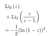
… ►For results, including error bounds, see Olver (1977c). ►For connection formulas for Liouville–Green approximations across these transition points see Olver (1977b, a, 1978). …8: 25.12 Polylogarithms
…
►In the complex plane has a branch point at .
…
►
25.12.3
.
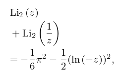
►
25.12.4
.
…
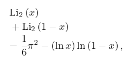
►
25.12.6
.
…
►Sometimes the factor is omitted.
…
9: 16.8 Differential Equations
…
►
§16.8(i) Classification of Singularities
►An ordinary point of the differential equation …If is not an ordinary point but , , are analytic at , then is a regular singularity. … ►When no is an integer, and no two differ by an integer, a fundamental set of solutions of (16.8.3) is given by … ►We have the connection formula …10: 19.2 Definitions
…
►The paths of integration are the line segments connecting the limits of integration.
The integral for is well defined if , and the Cauchy principal value (§1.4(v)) of is taken if vanishes at an interior point of the integration path.
…The circular and hyperbolic cases alternate in the four intervals of the real line separated by the points
.
…
►with a branch point at and principal branch .
…
►Let and .
…
