Schur parameters
(0.003 seconds)
1—10 of 386 matching pages
1: 18.33 Polynomials Orthogonal on the Unit Circle
…
►
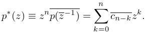
18.33.22
►The Verblunsky coefficients (also called Schur parameters or reflection coefficients) are the coefficients in the Szegő recurrence relations
…
2: Bibliography D
…
►
Accurate and efficient evaluation of Schur and Jack functions.
Math. Comp. 75 (253), pp. 223–239.
…
►
Uniform asymptotic expansions for prolate spheroidal functions with large parameters.
SIAM J. Math. Anal. 17 (6), pp. 1495–1524.
…
►
Conical functions with one or both parameters large.
Proc. Roy. Soc. Edinburgh Sect. A 119 (3-4), pp. 311–327.
►
Uniform asymptotic expansions for oblate spheroidal functions I: Positive separation parameter
.
Proc. Roy. Soc. Edinburgh Sect. A 121 (3-4), pp. 303–320.
…
►
Uniform asymptotic expansions for oblate spheroidal functions II: Negative separation parameter
.
Proc. Roy. Soc. Edinburgh Sect. A 125 (4), pp. 719–737.
…
3: Bibliography M
…
►
On one-parameter families of Painlevé III.
Stud. Appl. Math. 101 (3), pp. 321–341.
…
►
Fast computation of the Gauss hypergeometric function with all its parameters complex with application to the Pöschl-Teller-Ginocchio potential wave functions.
Comput. Phys. Comm. 178 (7), pp. 535–551.
…
►
Infinite families of exact sums of squares formulas, Jacobi elliptic functions, continued fractions, and Schur functions.
Ramanujan J. 6 (1), pp. 7–149.
…
►
The characteristic numbers of the Mathieu equation with purely imaginary parameter.
Phil. Mag. Series 7 8 (53), pp. 834–840.
…
►
Tables of the functions of the parabolic cylinder for negative integer parameters.
Zastos. Mat. 13, pp. 261–273.
…
4: 31.13 Asymptotic Approximations
§31.13 Asymptotic Approximations
►For asymptotic approximations for the accessory parameter eigenvalues , see Fedoryuk (1991) and Slavyanov (1996). …5: 31.3 Basic Solutions
6: 29.11 Lamé Wave Equation
…
►
29.11.1
►in which is another parameter.
…
►For properties of the solutions of (29.11.1) see Arscott (1956, 1959), Arscott (1964b, Chapter X), Erdélyi et al. (1955, §16.14), Fedoryuk (1989), and Müller (1966a, b, c).
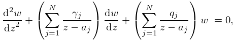
7: 31.14 General Fuchsian Equation
…
►
►The three sets of parameters comprise the singularity parameters
, the exponent parameters
, and the free accessory parameters
.
With and the total number of free parameters is .
…
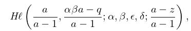
►
31.14.1
.
…
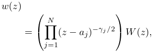
►
31.14.3
…
8: 28.17 Stability as
§28.17 Stability as
►If all solutions of (28.2.1) are bounded when along the real axis, then the corresponding pair of parameters is called stable. … ►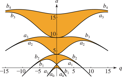 ►
►
9: 31.1 Special Notation
…
►
►
…
►Sometimes the parameters are suppressed.
| , | real variables. |
|---|---|
| … | |
| complex parameter, . | |
| complex parameters. | |
