Jacobi fraction (J-fraction)
(0.002 seconds)
11—20 of 217 matching pages
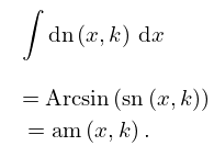
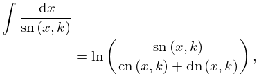
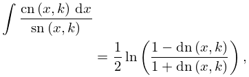
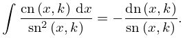
11: 18.17 Integrals
12: 22.4 Periods, Poles, and Zeros
…
►For example, the poles of , abbreviated as in the following tables, are at .
…
►Then: (a) In any lattice unit cell has a simple zero at and a simple pole at .
(b) The difference between p and the nearest q is a half-period of .
This half-period will be plus or minus a member of the triple ; the other two members of this triple are quarter periods of .
…
►For example, .
…
13: 20.4 Values at = 0
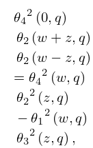
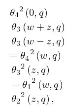
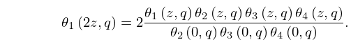
14: 20.7 Identities
15: 18.30 Associated OP’s
…
►Associated polynomials and the related corecursive polynomials appear in Ismail (2009, §§2.3, 2.6, and 2.10), where the relationship of OP’s to continued fractions is made evident.
…
►
§18.30(i) Associated Jacobi Polynomials
… ►For corresponding corecursive associated Jacobi polynomials, corecursive associated polynomials being discussed in §18.30(vii), see Letessier (1995). For other results for associated Jacobi polynomials, see Wimp (1987) and Ismail and Masson (1991). … ►See Ismail (2009, p. 46 ), where the th corecursive polynomial is also related to an appropriate continued fraction, given here as its th convergent, …16: 10.55 Continued Fractions
§10.55 Continued Fractions
►For continued fractions for and see Cuyt et al. (2008, pp. 350, 353, 362, 363, 367–369).17: 15.9 Relations to Other Functions
18: 22.1 Special Notation
…
►The functions treated in this chapter are the three principal Jacobian elliptic functions , , ; the nine subsidiary Jacobian elliptic functions , , , , , , , , ; the amplitude function ; Jacobi’s epsilon and zeta functions and .
…
►The notation , , is due to Gudermann (1838), following Jacobi (1827); that for the subsidiary functions is due to Glaisher (1882).
Other notations for are and with ; see Abramowitz and Stegun (1964) and Walker (1996).
…
19: 18.7 Interrelations and Limit Relations
…
►
