.2021世界杯投注_『wn4.com_』世界杯挣钱机遇_w6n2c9o_2022年12月2日21时22分29秒_f7zjzd5rf_gov_hk

(0.008 seconds)

21—30 of 850 matching pages

21: 16.10 Expansions in Series of ${{}_{p}F_{q}}$ Functions

§16.10 Expansions in Series of ${{}_{p}F_{q}}$ Functions

… ►

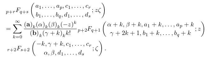
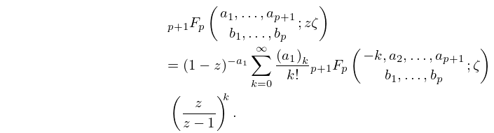
16.10.1

{{}_{p+r}F_{q+s}}\left({a_{1},\dots,a_{p},c_{1},\dots,c_{r}\atop b_{1},\dots,b% _{q},d_{1},\dots,d_{s}};z\zeta\right)=\sum_{k=0}^{\infty}\frac{{\left(\mathbf{% a}\right)_{k}}{\left(\alpha\right)_{k}}{\left(\beta\right)_{k}}(-z)^{k}}{{% \left(\mathbf{b}\right)_{k}}{\left(\gamma+k\right)_{k}}k!}{{}_{p+2}F_{q+1}}% \left({\alpha+k,\beta+k,a_{1}+k,\dots,a_{p}+k\atop\gamma+2k+1,b_{1}+k,\dots,b_% {q}+k};z\right){{}_{r+2}F_{s+2}}\left({-k,\gamma+k,c_{1},\dots,c_{r}\atop% \alpha,\beta,d_{1},\dots,d_{s}};\zeta\right).

ⓘ

Symbols:: ${{}_{\NVar{p}}F_{\NVar{q}}}\left(\NVar{a_{1},\dots,a_{p}};\NVar{b_{1},\dots,b_% {q}};\NVar{z}\right)$ or ${{}_{\NVar{p}}F_{\NVar{q}}}\left({\NVar{a_{1},\dots,a_{p}}\atop\NVar{b_{1},% \dots,b_{q}}};\NVar{z}\right)$ : alternatively ${{}_{\NVar{p}}F_{\NVar{q}}}\left(\NVar{\mathbf{a}};\NVar{\mathbf{b}};\NVar{z}\right)$ or ${{}_{\NVar{p}}F_{\NVar{q}}}\left({\NVar{\mathbf{a}}\atop\NVar{\mathbf{b}}};% \NVar{z}\right)$
generalized hypergeometric function, ${\left(\NVar{a}\right)_{\NVar{n}}}$ : Pochhammer’s symbol (or shifted factorial), $!$ : factorial (as in $n!$ ), $p$ : nonnegative integer, $q$ : nonnegative integer, $z$ : complex variable, $a,a_{1},\ldots,a_{p}$ : real or complex parameters and $b,b_{1},\ldots,b_{q}$ : real or complex parameters
Permalink:: http://dlmf.nist.gov/16.10.E1
Encodings:: pMML, png, TeX
See also:: Annotations for §16.10 and Ch.16

… ►

16.10.2

{{}_{p+1}F_{p}}\left({a_{1},\dots,a_{p+1}\atop b_{1},\dots,b_{p}};z\zeta\right% )=(1-z)^{-a_{1}}\sum_{k=0}^{\infty}\frac{{\left(a_{1}\right)_{k}}}{k!}{{}_{p+1% }F_{p}}\left({-k,a_{2},\dots,a_{p+1}\atop b_{1},\dots,b_{p}};\zeta\right)\left% (\frac{z}{z-1}\right)^{k}.

ⓘ

Symbols:: ${{}_{\NVar{p}}F_{\NVar{q}}}\left(\NVar{a_{1},\dots,a_{p}};\NVar{b_{1},\dots,b_% {q}};\NVar{z}\right)$ or ${{}_{\NVar{p}}F_{\NVar{q}}}\left({\NVar{a_{1},\dots,a_{p}}\atop\NVar{b_{1},% \dots,b_{q}}};\NVar{z}\right)$ : alternatively ${{}_{\NVar{p}}F_{\NVar{q}}}\left(\NVar{\mathbf{a}};\NVar{\mathbf{b}};\NVar{z}\right)$ or ${{}_{\NVar{p}}F_{\NVar{q}}}\left({\NVar{\mathbf{a}}\atop\NVar{\mathbf{b}}};% \NVar{z}\right)$
generalized hypergeometric function, ${\left(\NVar{a}\right)_{\NVar{n}}}$ : Pochhammer’s symbol (or shifted factorial), $!$ : factorial (as in $n!$ ), $p$ : nonnegative integer, $z$ : complex variable, $a,a_{1},\ldots,a_{p}$ : real or complex parameters and $b,b_{1},\ldots,b_{q}$ : real or complex parameters
Permalink:: http://dlmf.nist.gov/16.10.E2
Encodings:: pMML, png, TeX
See also:: Annotations for §16.10 and Ch.16

►When

|\zeta-1|<1

the series on the right-hand side converges in the half-plane

\Re z<\frac{1}{2}

. ►Expansions of the form

\sum_{n=1}^{\infty}(\pm 1)^{n}{{}_{p}F_{p+1}}\left(\mathbf{a};\mathbf{b};-n^{2% }z^{2}\right)

are discussed in Miller (1997), and further series of generalized hypergeometric functions are given in Luke (1969b, Chapter 9), Luke (1975, §§5.10.2 and 5.11), and Prudnikov et al. (1990, §§5.3, 6.8–6.9).

22: 1.12 Continued Fractions

… ►

b_{0}+\displaystyle{\cfrac{a_{1}}{b_{1}+\cfrac{a_{2}}{b_{2}+\cdots}}}

is equivalent to

b^{\prime}_{0}+\displaystyle{\cfrac{a^{\prime}_{1}}{b^{\prime}_{1}+\cfrac{a^{% \prime}_{2}}{b^{\prime}_{2}+\cdots}}}

if there is a sequence

\{d_{n}\}^{\infty}_{n=0}

d_{0}=1

d_{n}\neq 0

, such that … ►when

p_{k}\not=0

k=1,2,3,\dots

. …when

c_{k}\not=0

k=1,2,3,\dots

. … ►The continued fraction

\displaystyle{\cfrac{a_{1}}{b_{1}+\cfrac{a_{2}}{b_{2}+\cdots}}}

converges when … ►Let the elements of the continued fraction

\displaystyle{\cfrac{1}{b_{1}+\cfrac{1}{b_{2}+\cdots}}}

satisfy …

23: 3.6 Linear Difference Equations

… ►where

\Delta w_{n-1}=w_{n}-w_{n-1}

\Delta^{2}w_{n-1}=\Delta w_{n}-\Delta w_{n-1}

, and

n\in\mathbb{Z}

. … ►Stability can be restored, however, by backward recursion, provided that

c_{n}\neq 0

\forall n

: starting from

w_{N}

and

w_{N+1}

, with

N

large, equation (3.6.3) is applied to generate in succession

w_{N-1},w_{N-2},\dots,w_{0}

. … ►Let us assume the normalizing condition is of the form

w_{0}=\lambda

, where

\lambda

is a constant, and then solve the following tridiagonal system of algebraic equations for the unknowns

w_{1}^{(N)},w_{2}^{(N)},\dots,w_{N-1}^{(N)}

; see §3.2(ii). … ►Suppose again that

f_{0}\neq 0

w_{0}

is given, and we wish to calculate

w_{1},w_{2},\dots,w_{M}

to a prescribed relative accuracy

\epsilon

for a given value of

M

. … ►The values of

w_{n}

for

n=1,2,\dots,10

are the wanted values of

\mathbf{E}_{n}\left(1\right)

. …

24: 11.14 Tables

… ►

•

Abramowitz and Stegun (1964, Chapter 12) tabulates $\mathbf{H}_{n}\left(x\right)$ , $\mathbf{H}_{n}\left(x\right)-Y_{n}\left(x\right)$ , and $I_{n}\left(x\right)-\mathbf{L}_{n}\left(x\right)$ for $n=0,1$ and $x=0(.1)5$ , $x^{-1}=0(.01)0.2$ to 6D or 7D.

… ►

•

Abramowitz and Stegun (1964, Chapter 12) tabulates $\int_{0}^{x}(I_{0}\left(t\right)-\mathbf{L}_{0}\left(t\right))\,\mathrm{d}t$ and $(2/\pi)\int_{x}^{\infty}t^{-1}\mathbf{H}_{0}\left(t\right)\,\mathrm{d}t$ for $x=0(.1)5$ to 5D or 7D; $\int_{0}^{x}(\mathbf{H}_{0}\left(t\right)-Y_{0}\left(t\right))\,\mathrm{d}t-(2% /\pi)\ln x$ , $\int_{0}^{x}(I_{0}\left(t\right)-\mathbf{L}_{0}\left(t\right))\,\mathrm{d}t-(2% /\pi)\ln x$ , and $\int_{x}^{\infty}t^{-1}(\mathbf{H}_{0}\left(t\right)-Y_{0}\left(t\right))\,% \mathrm{d}t$ for $x^{-1}=0(.01)0.2$ to 6D.

►

•

Agrest et al. (1982) tabulates $\int_{0}^{x}\mathbf{H}_{0}\left(t\right)\,\mathrm{d}t$ and $e^{-x}\int_{0}^{x}\mathbf{L}_{0}\left(t\right)\,\mathrm{d}t$ for $x=0(.001)5(.005)15(.01)100$ to 11D.

… ►

•

Jahnke and Emde (1945) tabulates $\mathbf{E}_{n}\left(x\right)$ for $n=1,2$ and $x=0(.01)14.99$ to 4D.

… ►

•

Agrest and Maksimov (1971, Chapter 11) defines incomplete Struve, Anger, and Weber functions and includes tables of an incomplete Struve function $\mathbf{H}_{n}\left(x,\alpha\right)$ for $n=0,1$ , $x=0(.2)10$ , and $\alpha=0(.2)1.4,\tfrac{1}{2}\pi$ , together with surface plots.

25: 3.7 Ordinary Differential Equations

… ►The path is partitioned at

P+1

points labeled successively

z_{0},z_{1},\dots,z_{P}

, with

z_{0}=a

z_{P}=b

. … ►Let

\mathbf{A}_{P}

be the

(2P)\times(2P+2)

band matrix … ►This is a set of

2P

equations for the

2P+2

unknowns,

w(z_{j})

and

w^{\prime}(z_{j})

j=0,1,\dots,P

. … ►The values

\lambda_{k}

are the eigenvalues and the corresponding solutions

w_{k}

of the differential equation are the eigenfunctions. … ►where

h=z_{n+1}-z_{n}

and …

26: 3.9 Acceleration of Convergence

… ►Then the transformation of the sequence

\{s_{n}\}

into a sequence

\{t_{n,2k}\}

is given by … ►Then

t_{n,2k}=\varepsilon_{2k}^{(n)}

. … ►If

s_{n}

is the

n

th partial sum of a power series

f

, then

t_{n,2k}=\varepsilon_{2k}^{(n)}

is the Padé approximant

[(n+k)/k]_{f}

(§3.11(iv)). … ►In Table 3.9.1 values of the transforms

t_{n,2k}

are supplied for …with

s_{\infty}=\frac{1}{12}{\pi}^{2}=0.82246\;70334\;24\dotsc

. …

27: 13.22 Zeros

… ►From (13.14.2) and (13.14.3)

M_{\kappa,\mu}\left(z\right)

has the same zeros as

M\left(\tfrac{1}{2}+\mu-\kappa,1+2\mu,z\right)

and

W_{\kappa,\mu}\left(z\right)

has the same zeros as

U\left(\tfrac{1}{2}+\mu-\kappa,1+2\mu,z\right)

, hence the results given in §13.9 can be adopted. … ►For example, if

\mu(\geq 0)

is fixed and

\kappa(>0)

is large, then the

r

th positive zero

\phi_{r}

M_{\kappa,\mu}\left(z\right)

is given by ►

13.22.1

\phi_{r}=\frac{j_{2\mu,r}^{2}}{4\kappa}+j_{2\mu,r}O\left(\kappa^{-\frac{3}{2}}% \right),

ⓘ

Symbols:: $O\left(\NVar{x}\right)$ : order not exceeding, $\phi_{r}$ : positive zeros and $j_{b,r}$ : positive zero of Bessel
Referenced by:: §13.22, §13.22
Permalink:: http://dlmf.nist.gov/13.22.E1
Encodings:: pMML, png, TeX
See also:: Annotations for §13.22 and Ch.13

►where

j_{2\mu,r}

is the

r

th positive zero of the Bessel function

J_{2\mu}\left(x\right)

(§10.21(i)). …

28: 26.9 Integer Partitions: Restricted Number and Part Size

… ►

p_{k}\left(n\right)

denotes the number of partitions of

n

into at most

k

parts. See Table 26.9.1. … ►It follows that

p_{k}\left(n\right)

also equals the number of partitions of

n

into parts that are less than or equal to

k

. ►

p_{k}\left(\leq m,n\right)

is the number of partitions of

n

into at most

k

parts, each less than or equal to

m

. …

29: 28.6 Expansions for Small $q$

… ►Leading terms of the power series for

a_{m}\left(q\right)

and

b_{m}\left(q\right)

for

m\leq 6

are: … ►The coefficients of the power series of

a_{2n}\left(q\right)

b_{2n}\left(q\right)

and also

a_{2n+1}\left(q\right)

b_{2n+1}\left(q\right)

are the same until the terms in

q^{2n-2}

and

q^{2n}

, respectively. … ►Numerical values of the radii of convergence

\rho_{n}^{(j)}

of the power series (28.6.1)–(28.6.14) for

n=0,1,\dots,9

are given in Table 28.6.1. Here

j=1

for

a_{2n}\left(q\right)

j=2

for

b_{2n+2}\left(q\right)

, and

j=3

for

a_{2n+1}\left(q\right)

and

b_{2n+1}\left(q\right)

. … ►

§28.6(ii) Functions $\operatorname{ce}_{n}$ and $\operatorname{se}_{n}$

…

30: 20.4 Values at $z$ = 0

… ►

20.4.1

\theta_{1}\left(0,q\right)=\theta_{2}'\left(0,q\right)=\theta_{3}'\left(0,q% \right)=\theta_{4}'\left(0,q\right)=0,

ⓘ

Symbols:: $\theta_{\NVar{j}}\left(\NVar{z},\NVar{q}\right)$ : theta function and $q$ : nome
Permalink:: http://dlmf.nist.gov/20.4.E1
Encodings:: pMML, png, TeX
See also:: Annotations for §20.4(i), §20.4 and Ch.20

… ►

20.4.6

\theta_{1}'\left(0,q\right)=\theta_{2}\left(0,q\right)\theta_{3}\left(0,q% \right)\theta_{4}\left(0,q\right).

ⓘ

Symbols:: $\theta_{\NVar{j}}\left(\NVar{z},\NVar{q}\right)$ : theta function and $q$ : nome
A&S Ref:: 16.28.6
Referenced by:: §20.9(i)
Permalink:: http://dlmf.nist.gov/20.4.E6
Encodings:: pMML, png, TeX
See also:: Annotations for §20.4(i), §20.4(i), §20.4 and Ch.20

… ►

20.4.7

\theta_{1}''\left(0,q\right)=\theta_{2}'''\left(0,q\right)=\theta_{3}'''\left(% 0,q\right)=\theta_{4}'''\left(0,q\right)=0.

ⓘ

Symbols:: $\theta_{\NVar{j}}\left(\NVar{z},\NVar{q}\right)$ : theta function and $q$ : nome
Permalink:: http://dlmf.nist.gov/20.4.E7
Encodings:: pMML, png, TeX
See also:: Annotations for §20.4(ii), §20.4 and Ch.20

… ►

20.4.9

\frac{\theta_{2}''\left(0,q\right)}{\theta_{2}\left(0,q\right)}=-1-8\sum_{n=1}% ^{\infty}\frac{q^{2n}}{(1+q^{2n})^{2}},

ⓘ

Symbols:: $\theta_{\NVar{j}}\left(\NVar{z},\NVar{q}\right)$ : theta function, $n$ : integer and $q$ : nome
Permalink:: http://dlmf.nist.gov/20.4.E9
Encodings:: pMML, png, TeX
See also:: Annotations for §20.4(ii), §20.4 and Ch.20

… ►

20.4.12

\frac{\theta_{1}'''\left(0,q\right)}{\theta_{1}'\left(0,q\right)}=\frac{\theta% _{2}''\left(0,q\right)}{\theta_{2}\left(0,q\right)}+\frac{\theta_{3}''\left(0,% q\right)}{\theta_{3}\left(0,q\right)}+\frac{\theta_{4}''\left(0,q\right)}{% \theta_{4}\left(0,q\right)}.

ⓘ

Symbols:: $\theta_{\NVar{j}}\left(\NVar{z},\NVar{q}\right)$ : theta function and $q$ : nome
Permalink:: http://dlmf.nist.gov/20.4.E12
Encodings:: pMML, png, TeX
See also:: Annotations for §20.4(ii), §20.4 and Ch.20