change of modulus

SearchAdvancedHelp

(0.004 seconds)

31—40 of 92 matching pages

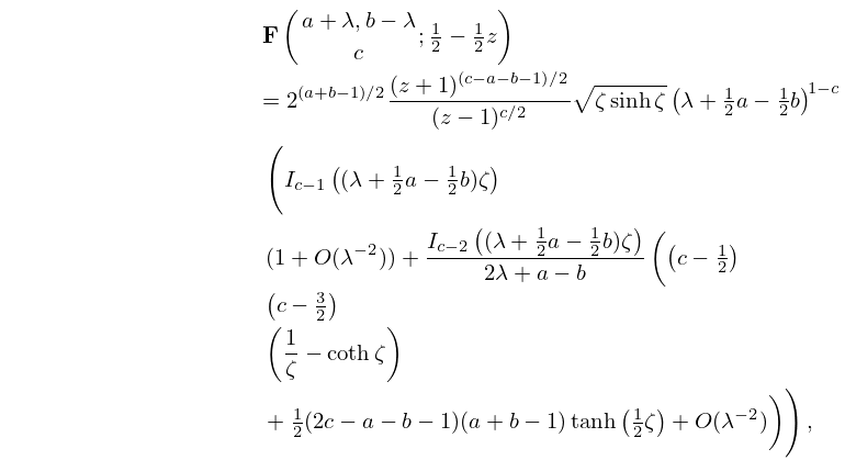
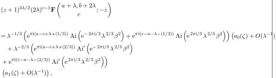
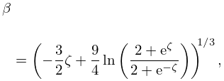
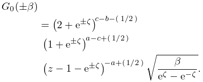
31: 15.12 Asymptotic Approximations

… ►

15.12.5 $$𝐅(\genfrac{}{}{0pt}{}{a+\lambda ,b-\lambda }{c};\frac{1}{2}-\frac{1}{2}z)=2^{(a+b-1)/2}\frac{{(z+1)}^{(c-a-b-1)/2}}{{(z-1)}^{c/2}}\sqrt{\zeta \sinh \zeta }{\left(\lambda +\frac{1}{2}a-\frac{1}{2}b\right)}^{1-c}\left(I_{c-1}\left((\lambda +\frac{1}{2}a-\frac{1}{2}b)\zeta \right)(1+O({\lambda }^{-2}))+\frac{I_{c-2}\left((\lambda +\frac{1}{2}a-\frac{1}{2}b)\zeta \right)}{2\lambda +a-b}\left(\left(c-\frac{1}{2}\right)\left(c-\frac{3}{2}\right)\left(\frac{1}{\zeta }-\coth \zeta \right)+\frac{1}{2}(2c-a-b-1)(a+b-1)\tanh \left(\frac{1}{2}\zeta \right)+O({\lambda }^{-2})\right)\right),$$

ⓘ

Symbols:

$O\left(x\right)$: order not exceeding, $\coth z$: hyperbolic cotangent function, $\sinh z$: hyperbolic sine function, $\tanh z$: hyperbolic tangent function, $I_{\nu }\left(z\right)$: modified Bessel function of the first kind, $𝐅(a,b;c;z)$ or $𝐅(\genfrac{}{}{0pt}{}{a,b}{c};z)$: $={}_2{}^{}𝐅_1^{}(a,b;c;z)$ Olver’s hypergeometric function, $z$: complex variable, $a$: real or complex parameter, $b$: real or complex parameter, $c$: real or complex parameter and $\zeta$: change of variable

Permalink:

http://dlmf.nist.gov/15.12.E5

Encodings:

pMML, png, TeX

See also:

Annotations for §15.12(iii), §15.12 and Ch.15

… ►

15.12.9 $${(z+1)}^{3\lambda /2}{(2\lambda )}^{c-1}𝐅(\genfrac{}{}{0pt}{}{a+\lambda ,b+2\lambda }{c};-z)={\lambda }^{-1/3}\left({\mathrm{e}}^{\pi \mathrm{i}(a-c+\lambda +(1/3))}\mathrm{Ai}\left({\mathrm{e}}^{-2\pi \mathrm{i}/3}{\lambda }^{2/3}{\beta }^2\right)+{\mathrm{e}}^{\pi \mathrm{i}(c-a-\lambda -(1/3))}\mathrm{Ai}\left({\mathrm{e}}^{2\pi \mathrm{i}/3}{\lambda }^{2/3}{\beta }^2\right)\right)\left(a_0(\zeta )+O({\lambda }^{-1})\right)+{\lambda }^{-2/3}\left({\mathrm{e}}^{\pi \mathrm{i}(a-c+\lambda +(2/3))}{\mathrm{Ai}}^{\prime }\left({\mathrm{e}}^{-2\pi \mathrm{i}/3}{\lambda }^{2/3}{\beta }^2\right)+{\mathrm{e}}^{\pi \mathrm{i}(c-a-\lambda -(2/3))}{\mathrm{Ai}}^{\prime }\left({\mathrm{e}}^{2\pi \mathrm{i}/3}{\lambda }^{2/3}{\beta }^2\right)\right)\left(a_1(\zeta )+O({\lambda }^{-1})\right),$$

ⓘ

Symbols:

$\mathrm{Ai}\left(z\right)$: Airy function, $O\left(x\right)$: order not exceeding, $\pi$: the ratio of the circumference of a circle to its diameter, $\mathrm{e}$: base of natural logarithm, $\mathrm{i}$: imaginary unit, $𝐅(a,b;c;z)$ or $𝐅(\genfrac{}{}{0pt}{}{a,b}{c};z)$: $={}_2{}^{}𝐅_1^{}(a,b;c;z)$ Olver’s hypergeometric function, $z$: complex variable, $a$: real or complex parameter, $b$: real or complex parameter, $c$: real or complex parameter, $\zeta$: change of variable, $\beta$ and $a_j(\zeta )$: function

Referenced by:

§15.12(iii)

Permalink:

http://dlmf.nist.gov/15.12.E9

Encodings:

pMML, png, TeX

See also:

Annotations for §15.12(iii), §15.12 and Ch.15

… ►

15.12.11 $$\beta ={\left(-\frac{3}{2}\zeta +\frac{9}{4}\ln \left(\frac{2+{\mathrm{e}}^{\zeta }}{2+{\mathrm{e}}^{-\zeta }}\right)\right)}^{1/3},$$

ⓘ

Symbols:

$\mathrm{e}$: base of natural logarithm, $\ln z$: principal branch of logarithm function, $\zeta$: change of variable and $\beta$

Permalink:

http://dlmf.nist.gov/15.12.E11

Encodings:

pMML, png, TeX

See also:

Annotations for §15.12(iii), §15.12 and Ch.15

… ►

15.12.13 $$G_0(\pm \beta )={\left(2+{\mathrm{e}}^{\pm \zeta }\right)}^{c-b-(1/2)}{\left(1+{\mathrm{e}}^{\pm \zeta }\right)}^{a-c+(1/2)}{\left(z-1-{\mathrm{e}}^{\pm \zeta }\right)}^{-a+(1/2)}\sqrt{\frac{\beta }{{\mathrm{e}}^{\zeta }-{\mathrm{e}}^{-\zeta }}}.$$

ⓘ

Symbols:

$\mathrm{e}$: base of natural logarithm, $z$: complex variable, $a$: real or complex parameter, $b$: real or complex parameter, $c$: real or complex parameter, $\zeta$: change of variable, $\beta$ and $G_0(\pm \zeta )$: function

Permalink:

http://dlmf.nist.gov/15.12.E13

Encodings:

pMML, png, TeX

See also:

Annotations for §15.12(iii), §15.12 and Ch.15

…

32: 19.2 Definitions

… ►The cases with $\varphi =\pi /2$ are the complete integrals: … ►

$k_c=k^{\prime },$

►

$p=1-{\alpha }^2,$

►

$x=\tan \varphi ,$

… ►If , then $k_c$ is pure imaginary. …

33: 2.11 Remainder Terms; Stokes Phenomenon

… ►In the transition through $\theta =\pi$, $\mathrm{erfc}\left(\sqrt{\frac{1}{2}\rho }c(\theta )\right)$ changes very rapidly, but smoothly, from one form to the other; compare the graph of its modulus in Figure 2.11.1 in the case $\rho =100$. …

34: 2.4 Contour Integrals

… ►

2.4.20 $$f(\alpha ,w)=q(\alpha ,t)\frac{dt}{dw}=q(\alpha ,t)\frac{w^2+2aw+b}{\partial p(\alpha ,t)/\partial t}.$$

ⓘ

Symbols:

$\frac{df}{dx}$: derivative of $f$ with respect to $x$ , $\frac{\partial f}{\partial x}$: partial derivative of $f$ with respect to $x$ , $\partial x$: partial differential of $x$ , $p(t)$: analytic function, $q(t)$: analytic function, $w$: change of variable, $a$ , $b$ and $f(\alpha ,w)$: function

Permalink:

http://dlmf.nist.gov/2.4.E20

Encodings:

pMML, png, TeX

See also:

Annotations for §2.4(v), §2.4 and Ch.2

… ►

2.4.21 $$w=z^{-1/3}v-a,$$

ⓘ

Symbols:

$w$: change of variable and $a$

Referenced by:

§2.4(v)

Permalink:

http://dlmf.nist.gov/2.4.E21

Encodings:

pMML, png, TeX

See also:

Annotations for §2.4(v), §2.4 and Ch.2

…

35: 7.7 Integral Representations

… ►

7.7.13 $$\mathrm{f}\left(z\right)=\frac{{(2\pi )}^{-3/2}}{2\pi \mathrm{i}}{\int }_{c-\mathrm{i}\mathrm{\infty }}^{c+\mathrm{i}\mathrm{\infty }}{\zeta }^{-s}\mathrm{\Gamma }\left(s\right)\mathrm{\Gamma }\left(s+\frac{1}{2}\right)\mathrm{\Gamma }\left(s+\frac{3}{4}\right)\mathrm{\Gamma }\left(\frac{1}{4}-s\right)ds,$$

ⓘ

Symbols:

$\mathrm{\Gamma }\left(z\right)$: gamma function, $\mathrm{f}\left(z\right)$: auxiliary function for Fresnel integrals, $\pi$: the ratio of the circumference of a circle to its diameter, $dx$: differential of $x$ , $\mathrm{i}$: imaginary unit, $\int$: integral, $z$: complex variable, $\zeta$: change of variable and $c$: constant

Keywords:

Mellin transform

Referenced by:

§7.7(ii), §7.7(ii)

Permalink:

http://dlmf.nist.gov/7.7.E13

Encodings:

pMML, png, TeX

See also:

Annotations for §7.7(ii), §7.7(ii), §7.7 and Ch.7

►

7.7.14 $$\mathrm{g}\left(z\right)=\frac{{(2\pi )}^{-3/2}}{2\pi \mathrm{i}}{\int }_{c-\mathrm{i}\mathrm{\infty }}^{c+\mathrm{i}\mathrm{\infty }}{\zeta }^{-s}\mathrm{\Gamma }\left(s\right)\mathrm{\Gamma }\left(s+\frac{1}{2}\right)\mathrm{\Gamma }\left(s+\frac{1}{4}\right)\mathrm{\Gamma }\left(\frac{3}{4}-s\right)ds.$$

ⓘ

Symbols:

$\mathrm{\Gamma }\left(z\right)$: gamma function, $\mathrm{g}\left(z\right)$: auxiliary function for Fresnel integrals, $\pi$: the ratio of the circumference of a circle to its diameter, $dx$: differential of $x$ , $\mathrm{i}$: imaginary unit, $\int$: integral, $z$: complex variable, $\zeta$: change of variable and $c$: constant

Keywords:

Mellin transform

Referenced by:

§7.7(ii), §7.7(ii)

Permalink:

http://dlmf.nist.gov/7.7.E14

Encodings:

pMML, png, TeX

See also:

Annotations for §7.7(ii), §7.7(ii), §7.7 and Ch.7

…

36: 28.12 Definitions and Basic Properties

… ►For change of signs of $\nu$ and $q$, … ►For changes of sign of $\nu$, $q$, and $z$, … ►

28.12.9 $${\mathrm{me}}_{\nu }(z,-q)={\mathrm{e}}^{\mathrm{i}\nu \pi /2}{\mathrm{me}}_{\nu }(z-\frac{1}{2}\pi ,q),$$

ⓘ

Symbols:

${\mathrm{me}}_n(z,q)$: Mathieu function, $\pi$: the ratio of the circumference of a circle to its diameter, $\mathrm{e}$: base of natural logarithm, $\mathrm{i}$: imaginary unit, $q=h^2$: parameter, $z$: complex variable and $\nu$: complex parameter

Permalink:

http://dlmf.nist.gov/28.12.E9

Encodings:

pMML, png, TeX

See also:

Annotations for §28.12(ii), §28.12 and Ch.28

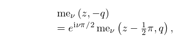
… ►When $\nu =s/m$ is a rational number, but not an integer, all solutions of Mathieu’s equation are periodic with period $2m\pi$. ►For change of signs of $\nu$ and $z$, …

37: 23.21 Physical Applications

… ►

23.21.3 $$f(\rho )=2{\left((\rho -e_1)(\rho -e_2)(\rho -e_3)\right)}^{1/2}.$$

ⓘ

Symbols:

$e_j$: Weierstrass lattice roots, $𝕃$: lattice, $\rho$: roots and $f(\rho )$: function

Permalink:

http://dlmf.nist.gov/23.21.E3

Encodings:

pMML, png, TeX

See also:

Annotations for §23.21(iii), §23.21 and Ch.23

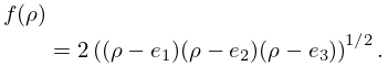
►Another form is obtained by identifying $e_1$, $e_2$, $e_3$ as lattice roots (§23.3(i)), and setting … ►

23.21.5 $$\left(\mathrm{\wp }\left(v\right)-\mathrm{\wp }\left(w\right)\right)\left(\mathrm{\wp }\left(w\right)-\mathrm{\wp }\left(u\right)\right)\left(\mathrm{\wp }\left(u\right)-\mathrm{\wp }\left(v\right)\right){\nabla }^2=\left(\mathrm{\wp }\left(w\right)-\mathrm{\wp }\left(v\right)\right)\frac{{\partial }^2}{{\partial u}^2}+\left(\mathrm{\wp }\left(u\right)-\mathrm{\wp }\left(w\right)\right)\frac{{\partial }^2}{{\partial v}^2}+\left(\mathrm{\wp }\left(v\right)-\mathrm{\wp }\left(u\right)\right)\frac{{\partial }^2}{{\partial w}^2}.$$

ⓘ

Symbols:

$\mathrm{\wp }\left(z\right)$ (= $\mathrm{\wp }\left(z|𝕃\right)$ = $\mathrm{\wp }(z;g_2,g_3)$): Weierstrass $\mathrm{\wp }$-function, $\frac{\partial f}{\partial x}$: partial derivative of $f$ with respect to $x$ , $\partial x$: partial differential of $x$ , $𝕃$: lattice, $u$: change of variable, $v$: change of variable and $w$: change of variable

Permalink:

http://dlmf.nist.gov/23.21.E5

Encodings:

pMML, png, TeX

See also:

Annotations for §23.21(iii), §23.21 and Ch.23

…

38: 2.3 Integrals of a Real Variable

… ►

2.3.12 $${\int }_0^{\mathrm{\infty }}f(xt)q(t)dt\sim \sum _{s=0}^{\mathrm{\infty }}ℳf\left(\frac{s+\lambda }{\mu }\right)\frac{a_s}{x^{(s+\lambda )/\mu }},$$ $x\to +\mathrm{\infty }$,

ⓘ

Symbols:

$ℳ\left(f\right)\left(s\right)$: Mellin transform, $\sim$: Poincaré asymptotic expansion, $dx$: differential of $x$ , $\int$: integral, $f(x)$: function, $a$: positive constant, $q(t)$: function, $\lambda$: positive constant and $\mu$: positive constant

Referenced by:

§2.3(ii), §2.3(ii)

Permalink:

http://dlmf.nist.gov/2.3.E12

Encodings:

pMML, png, TeX

Notational Change (effective with 1.0.15):

The notation for the Mellin transform was changed to $ℳf\left(s\right)$ from $ℳ(f;s)$.

See also:

Annotations for §2.3(ii), §2.3 and Ch.2

… ►

2.3.27 $$w={(2p(\alpha ,0)-2p(\alpha ,\alpha ))}^{1/2}\pm {(2p(\alpha ,t)-2p(\alpha ,\alpha ))}^{1/2},$$

ⓘ

Symbols:

$p(\alpha ,t)$: function and $w$: change of variable

Permalink:

http://dlmf.nist.gov/2.3.E27

Encodings:

pMML, png, TeX

See also:

Annotations for §2.3(v), §2.3 and Ch.2

… ►

2.3.28 $$\frac{dw}{dt}=\pm \frac{1}{{(2p(\alpha ,t)-2p(\alpha ,\alpha ))}^{1/2}}\frac{\partial p(\alpha ,t)}{\partial t}$$

ⓘ

Symbols:

$\frac{df}{dx}$: derivative of $f$ with respect to $x$ , $\frac{\partial f}{\partial x}$: partial derivative of $f$ with respect to $x$ , $\partial x$: partial differential of $x$ , $p(\alpha ,t)$: function and $w$: change of variable

Permalink:

http://dlmf.nist.gov/2.3.E28

Encodings:

pMML, png, TeX

See also:

Annotations for §2.3(v), §2.3 and Ch.2

…

39: 25.10 Zeros

… ►Because $|Z(t)|=|\zeta \left(\frac{1}{2}+\mathrm{i}t\right)|$, $Z(t)$ vanishes at the zeros of $\zeta \left(\frac{1}{2}+\mathrm{i}t\right)$, which can be separated by observing sign changes of $Z(t)$. Because $Z(t)$ changes sign infinitely often, $\zeta \left(\frac{1}{2}+\mathrm{i}t\right)$ has infinitely many zeros with $t$ real. … ►By comparing $N(T)$ with the number of sign changes of $Z(t)$ we can decide whether $\zeta \left(s\right)$ has any zeros off the line in this region. Sign changes of $Z(t)$ are determined by multiplying (25.9.3) by $\exp \left(\mathrm{i}\vartheta (t)\right)$ to obtain the Riemann–Siegel formula: …where $R(t)=O\left(t^{-1/4}\right)$ as $t\to \mathrm{\infty }$. …

40: 2.8 Differential Equations with a Parameter

… ►

2.8.2 $$W={\dot{z}}^{-1/2}w,$$

ⓘ

Symbols:

$w$: solution, $W$: change of variable and $\dot{z}$: derivative of $z$ with respect to $\xi$

Permalink:

http://dlmf.nist.gov/2.8.E2

Encodings:

pMML, png, TeX

See also:

Annotations for §2.8(i), §2.8 and Ch.2

… ►

2.8.8 $$d^{2}W/{d\xi }^2=\left(u^2{\xi }^m+\psi (\xi )\right)W,$$

ⓘ

Symbols:

$\frac{df}{dx}$: derivative of $f$ with respect to $x$ , $u$: large real or complex parameter, $W$: change of variable and $\psi (\xi )$: function

Referenced by:

§2.8(i), §2.8(iv)

Permalink:

http://dlmf.nist.gov/2.8.E8

Encodings:

pMML, png, TeX

See also:

Annotations for §2.8(i), §2.8 and Ch.2

…