discrete q-Hermite I and II polynomials

SearchAdvancedHelp

(0.002 seconds)

1—10 of 134 matching pages

1: 18.1 Notation

… ►

Discrete $q$-Hermite I: $h_n(x;q)$.

►

Discrete $q$-Hermite II: ${\tilde{h}}_n(x;q)$.

…

2: 18.27 $q$-Hahn Class

… ►

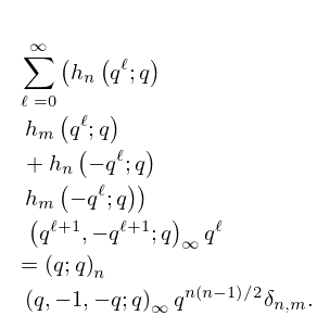
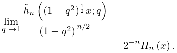
§18.27(vii) Discrete $q$-Hermite I and II Polynomials

… ►

18.27.22 $$\sum _{\mathrm{\ell }=0}^{\mathrm{\infty }}\left(h_n(q^{\mathrm{\ell }};q)h_m(q^{\mathrm{\ell }};q)+h_n(-q^{\mathrm{\ell }};q)h_m(-q^{\mathrm{\ell }};q)\right){(q^{\mathrm{\ell }+1},-q^{\mathrm{\ell }+1};q)}_{\mathrm{\infty }}{q}^{\mathrm{\ell }}={(q;q)}_n{(q,-1,-q;q)}_{\mathrm{\infty }}{q}^{n(n-1)/2}{\delta }_{n,m}.$$

ⓘ

Symbols:

${\delta }_{j,k}$: Kronecker delta, $h_n(x;q)$: discrete $q$-Hermite I polynomial, ${(a;q)}_n$: $q$-Pochhammer symbol (or $q$-shifted factorial), ${(a_1,a_2,\mathrm{\dots },a_r;q)}_n$: multiple $q$-Pochhammer symbol, $q$: real variable, $\mathrm{\ell }$: nonnegative integer, $m$: nonnegative integer and $n$: nonnegative integer

Permalink:

http://dlmf.nist.gov/18.27.E22

Encodings:

pMML, png, TeX

See also:

Annotations for §18.27(vii), §18.27(vii), §18.27 and Ch.18

►

Discrete $q$-Hermite II

… ►For discrete $q$-Hermite II polynomials the measure is not uniquely determined. … ►

18.27.26 $$\underset{q\to 1}{lim}\frac{{\tilde{h}}_n({(1-q^2)}^{\frac{1}{2}}x;q)}{{\left(1-q^2\right)}^{n/2}}=2^{-n}{H}_n\left(x\right).$$

ⓘ

Symbols:

$H_n\left(x\right)$: Hermite polynomial, ${\tilde{h}}_n(x;q)$: discrete $q$-Hermite II polynomial, $q$: real variable, $n$: nonnegative integer and $x$: real variable

Source:

Koekoek et al. (2010, (14.29.14))

Referenced by:

§18.27(vii), §18.27(vii), Erratum (V1.2.0) Section 18.27

Permalink:

http://dlmf.nist.gov/18.27.E26

Encodings:

pMML, png, TeX

Addition (effective with 1.2.0):

This equation was added.

See also:

Annotations for §18.27(vii), §18.27(vii), §18.27 and Ch.18

3: 18.3 Definitions

… ►In addition to the orthogonal property given by Table 18.3.1, the Chebyshev polynomials $T_n\left(x\right)$, $n=0,1,\mathrm{\dots },N$, are orthogonal on the discrete point set comprising the zeros $x_{N+1,n},n=1,2,\mathrm{\dots },N+1$, of $T_{N+1}\left(x\right)$: … ►For another version of the discrete orthogonality property of the polynomials $T_n\left(x\right)$ see (3.11.9). …

4: Bibliography H

… ►

A fast FFT-based discrete Legendre transform. IMA J. Numer. Anal. 36 (4), pp. 1670–1684.

ⓘ

External Links:

ISSN 0272-4979, Document, Link, MathReview (Denis N. Sidorov)

Referenced by:

§18.16(iii).

Encodings:

BibTeX

… ►

Algorithm 571: Statistics for von Mises’ and Fisher’s distributions of directions: $I_1(x)/I_0(x)$, $I_{1.5}(x)/I_{0.5}(x)$ and their inverses [S14]. ACM Trans. Math. Software 7 (2), pp. 233–238.

ⓘ

Notes:

Single-precision Fortran, minimum accuracy 8S.

External Links:

ISSN 0098-3500, Document, GAMS (module 571; package TOMS)

Referenced by:

5th item.

Encodings:

BibTeX

… ►

Roots of the Euler polynomials. Pacific J. Math. 64 (1), pp. 181–191.

ⓘ

External Links:

MathReview (M. Marden), ZentralBlatt

Referenced by:

§24.12(ii).

Encodings:

BibTeX

►

Explicit formulas for degenerate Bernoulli numbers. Discrete Math. 162 (1-3), pp. 175–185.

ⓘ

External Links:

ISSN 0012-365X, Document, MathReview (L. Skula), ZentralBlatt

Referenced by:

§24.16(i).

Encodings:

BibTeX

… ►

Bernoulli numbers and polynomials via residues. J. Number Theory 76 (2), pp. 178–193.

ⓘ

External Links:

ISSN 0022-314X, Document, MathReview (L. Skula), ZentralBlatt

Referenced by:

§24.14(ii).

Encodings:

BibTeX

…

5: 18.38 Mathematical Applications

… ►

Quadrature “Extended” to Pseudo-Spectral (DVR) Representations of Operators in One and Many Dimensions

…

6: 1.18 Linear Second Order Differential Operators and Eigenfunction Expansions

… ►

1.18.20 $${\delta }_{n,m}={\int }_a^b{\varphi }_n(x)\overline{{\varphi }_m(x)}dx.$$

ⓘ

Symbols:

${\delta }_{j,k}$: Kronecker delta, $\overline{z}$: complex conjugate, $dx$: differential of $x$ , $\int$: integral, $m$: nonnegative integer and $n$: nonnegative integer

Referenced by:

§1.18(v), §1.18(vi), §1.18(vi)

Permalink:

http://dlmf.nist.gov/1.18.E20

Encodings:

pMML, png, TeX

See also:

Annotations for §1.18(ii), §1.18 and Ch.1

…

7: 18.19 Hahn Class: Definitions

§18.19 Hahn Class: Definitions

►The Askey scheme extends the three families of classical OP’s (Jacobi, Laguerre and Hermite) with eight further families of OP’s for which the role of the differentiation operator $\frac{d}{dx}$ in the case of the classical OP’s is played by a suitable difference operator. … ►

Hahn class (or linear lattice class). These are OP’s $p_n(x)$ where the role of $\frac{d}{dx}$ is played by ${\mathrm{\Delta }}_x$ or ${\nabla }_x$ or ${\delta }_x$ (see §18.1(i) for the definition of these operators). The Hahn class consists of four discrete and two continuous families.

… ►The Hahn class consists of four discrete families (Hahn, Krawtchouk, Meixner, and Charlier) and two continuous families (continuous Hahn and Meixner–Pollaczek). … ►Tables 18.19.1 and 18.19.2 provide definitions via orthogonality and standardization (§§18.2(i), 18.2(iii)) for the Hahn polynomials $Q_n(x;\alpha ,\beta ,N)$, Krawtchouk polynomials $K_n(x;p,N)$, Meixner polynomials $M_n(x;\beta ,c)$, and Charlier polynomials $C_n(x;a)$. …

8: 18.35 Pollaczek Polynomials

§18.35 Pollaczek Polynomials

… ►There are 3 types of Pollaczek polynomials: … ►For the monic polynomials … ►

§18.35(ii) Orthogonality

… ►where, depending on $a,b,\lambda$, $D$ is a discrete subset of $ℝ$ and the $w_{\zeta }^{(\lambda )}(a,b)$ are certain weights. …

9: 18.39 Applications in the Physical Sciences

… ►

$w_{x_k}^{\mathrm{CP}}={\displaystyle \frac{(l+1+\frac{2Z}{s}){\rho }^{2k-1}{\left(1-{\rho }^2\right)}^{2l+3}{\left(2l+2\right)}_k}{2(k+l+1)k!}}.$

… ►

Discretized and Continuum Expansions of Scattering Eigenfunctions in terms of Pollaczek Polynomials: J-matrix Theory

…

10: 18.18 Sums

… ►

18.18.27 $$\sum _{n=0}^{\mathrm{\infty }}\frac{n!L_n^{(\alpha )}\left(x\right)L_n^{(\alpha )}\left(y\right)}{{\left(\alpha +1\right)}_n}{z}^n=\frac{\mathrm{\Gamma }\left(\alpha +1\right){(xyz)}^{-\frac{1}{2}\alpha }}{1-z}\exp \left(\frac{-(x+y)z}{1-z}\right)I_{\alpha }\left(\frac{2{(xyz)}^{\frac{1}{2}}}{1-z}\right),$$ .

ⓘ

Symbols:

$\mathrm{\Gamma }\left(z\right)$: gamma function, $L_n^{(\alpha )}\left(x\right)$: Laguerre (or generalized Laguerre) polynomial, ${\left(a\right)}_n$: Pochhammer’s symbol (or shifted factorial), $\exp z$: exponential function, $!$: factorial (as in $n!$), $I_{\nu }\left(z\right)$: modified Bessel function of the first kind, $y$: real variable, $z$: complex variable, $n$: nonnegative integer and $x$: real variable

Referenced by:

§18.18(vii), §18.18(vii)

Permalink:

http://dlmf.nist.gov/18.18.E27

Encodings:

pMML, png, TeX

See also:

Annotations for §18.18(vii), §18.18(vii), §18.18 and Ch.18

►For the modified Bessel function $I_{\nu }\left(z\right)$ see §10.25(ii). …