§1.16 Distributions
Contents
- §1.16(i) Test Functions
- §1.16(ii) Derivatives of a Distribution
- §1.16(iii) Dirac Delta Distribution
- §1.16(iv) Heaviside Function
- §1.16(v) Tempered Distributions
- §1.16(vi) Distributions of Several Variables
- §1.16(vii) Fourier Transforms of Tempered Distributions
- §1.16(viii) Fourier Transforms of Special Distributions
- §1.16(ix) References for Section 1.16
§1.16(i) Test Functions
Let be a function defined on an open interval , which can be infinite. The closure of the set of points where is called the support of . If the support of is a compact set (§1.9(vii)), then is called a function of compact support. A test function is an infinitely differentiable function of compact support.
A sequence of test functions converges to a test function if the support of every is contained in a fixed compact set and as the sequence converges uniformly on to for .
The linear space of all test functions with the above definition of convergence is called a test function space. We denote it by .
A mapping is a linear functional if
| 1.16.1 | |||
where and are real or complex constants. is called a distribution, or generalized function, if it is a continuous linear functional on , that is, it is a linear functional and for every in ,
| 1.16.2 | |||
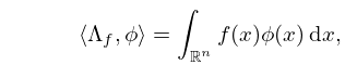
From here on we write for . The space of all distributions will be denoted by . A distribution is called regular if there is a locally integrable function on (i.e., a function on which is absolutely Lebesgue integrable on every compact subset of ) such that
| 1.16.3 | |||
We denote a regular distribution by , or simply , where is the function giving rise to the distribution. (If a distribution is not regular, it is called singular.) More generally, for a nondecreasing function the corresponding Lebesgue–Stieltjes measure (see §1.4(v)) can be considered as a distribution:
| 1.16.3_5 | |||
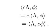
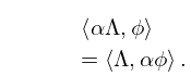
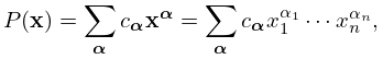
Define
| 1.16.4 | |||
| 1.16.5 | |||
where is a constant. More generally, if is an infinitely differentiable function, then
| 1.16.6 | |||
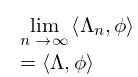
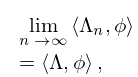
We say that a sequence of distributions converges to a distribution in if
| 1.16.7 | |||
for all .
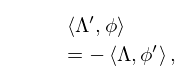
§1.16(ii) Derivatives of a Distribution
§1.16(iii) Dirac Delta Distribution
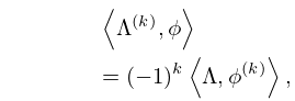
| 1.16.10 | ||||
| , | ||||
| 1.16.11 | ||||
| , | ||||
| 1.16.12 | ||||
| . | ||||
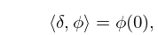
The Dirac delta distribution is singular. See also §1.17(i).
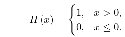
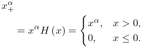
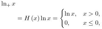
§1.16(iv) Heaviside Function
| 1.16.13 | ||||
| 1.16.14 | ||||
| 1.16.15 | ||||
| 1.16.16 | ||||
Since is the Lebesgue–Stieltjes measure corresponding to (see §1.4(v)), formula (1.16.16) is a special case of (1.16.3_5), (1.16.9_5) for that choice of .
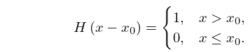
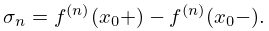
Suppose is infinitely differentiable except at , where left and right derivatives of all orders exist, and
| 1.16.17 | |||
Then
| 1.16.18 | |||
| . | |||
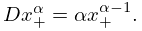
For ,
| 1.16.19 | |||
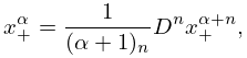
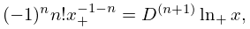
For ,
| 1.16.20 | |||
For and not an integer, define
| 1.16.21 | |||
where is an integer such that . Similarly, we write
| 1.16.22 | |||
and define
| 1.16.23 | |||
| . | |||
§1.16(v) Tempered Distributions
The space of test functions for tempered distributions consists of all infinitely-differentiable functions such that the function and all its derivatives are as for all .
A sequence of functions in is said to converge to a function as if the sequence converges uniformly to on every finite interval and if the constants in the inequalities
| 1.16.24 | |||
do not depend on .
A tempered distribution is a continuous linear functional on . (See the definition of a distribution in §1.16(i).) The set of tempered distributions is denoted by .
A sequence of tempered distributions converges to in if
| 1.16.25 | |||
for all .
The derivatives of tempered distributions are defined in the same way as derivatives of distributions.
For a detailed discussion of tempered distributions see Lighthill (1958).
§1.16(vi) Distributions of Several Variables
Let be the set of all infinitely differentiable functions in variables, , with compact support in . If is a multi-index and , then we write and . A sequence of functions in converges to a function if the supports of lie in a fixed compact subset of and converges uniformly to in for every multi-index . A distribution in is a continuous linear functional on .
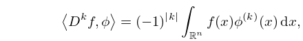
The partial derivatives of distributions in can be defined as in §1.16(ii). A locally integrable function gives rise to a distribution defined by
| 1.16.26 | |||
| . | |||
The distributional derivative of is defined by
| 1.16.27 | |||
| , | |||
where is a multi-index and .
For tempered distributions the space of test functions is the set of all infinitely-differentiable functions of variables that satisfy
| 1.16.28 | |||
| . | |||
Here and are multi-indices, and are constants. Tempered distributions are continuous linear functionals on this space of test functions. The space of tempered distributions is denoted by .
§1.16(vii) Fourier Transforms of Tempered Distributions
Suppose is a test function in . Then its Fourier transform is
| 1.16.29 | |||
where and . is also in .
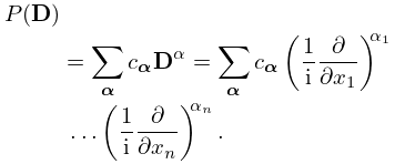
Let
| 1.16.30 | |||
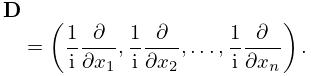
For a multi-index , define
| 1.16.31 | |||
and
| 1.16.32 | |||
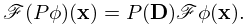
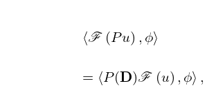
Here ranges over a finite set of multi-indices, is a multivariate polynomial, and is a partial differential operator. Then
| 1.16.33 | |||
and
| 1.16.34 | |||
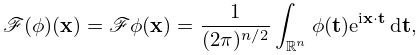
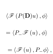
If is a tempered distribution, then its Fourier transform is defined by
| 1.16.35 | |||
| . | |||
The Fourier transform of a tempered distribution is again a tempered distribution, and
| 1.16.36 | |||
| 1.16.37 | |||
in which ; compare (1.16.33) and (1.16.34). In (1.16.36) and (1.16.37) the derivatives in are understood to be in the sense of distributions, as defined in §1.16(ii) and we also use the convention (1.16.6).
§1.16(viii) Fourier Transforms of Special Distributions
We use the notation of the previous subsection and take and in (1.16.35). We obtain
| 1.16.38 | |||
| . | |||
As distributions, the last equation reads
| 1.16.39 | |||
which is often written conventionally as
| 1.16.40 | |||
see also (1.17.2).
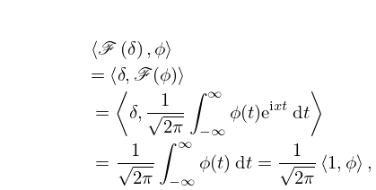
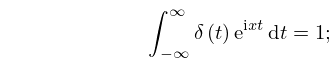
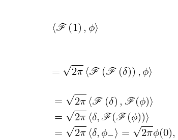
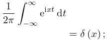
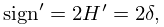
Since , we have
| 1.16.41 | |||
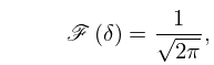
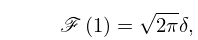
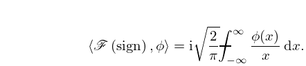
in which . The second to last equality follows from the Fourier integral formula (1.17.8). Since the quantity on the extreme right of (1.16.41) is equal to , as distributions, the result in this equation can be stated as
| 1.16.42 | |||
and conventionally it is expressed as
| 1.16.43 | |||
see also (1.17.12).
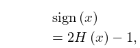
It is easily verified that
| 1.16.44 | |||
| , | |||
and from (1.16.15) we find
| 1.16.45 | |||
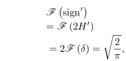
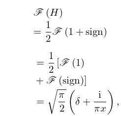
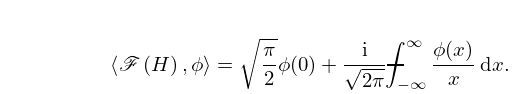
where is the Heaviside function defined in (1.16.13), and the derivatives are to be understood in the sense of distributions. Then
| 1.16.46 | |||
and from (1.16.36) with , , and , we have also
| 1.16.47 | |||
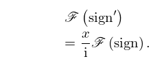
Coupling (1.16.46) and (1.16.47) gives
| 1.16.48 | |||
that is
| 1.16.49 | |||
§1.16(ix) References for Section 1.16
See Hildebrandt (1938) and Chihara (1978, Chapter II) for Stieltjes measures which are used in §18.39(iii); see also Shohat and Tamarkin (1970, Chapter II). Friedman (1990) gives an overview of generalized functions and their relation to distributions. See also Lighthill (1958), and Zemanian (1987).
