Heine%20transformations%20%28first%2C%20second%2C%20third%29

SearchAdvancedHelp

(0.011 seconds)

11—20 of 858 matching pages

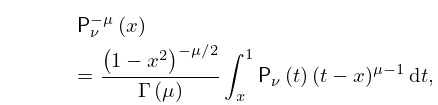
11: 14.12 Integral Representations

… ►

14.12.2 $${𝖯}_{\nu }^{-\mu }\left(x\right)=\frac{{\left(1-x^2\right)}^{-\mu /2}}{\mathrm{\Gamma }\left(\mu \right)}{\int }_x^1{𝖯}_{\nu }\left(t\right){(t-x)}^{\mu -1}dt,$$ $\mathrm{\Re }\mu >0$;

ⓘ

Symbols:

$\mathrm{\Gamma }\left(z\right)$: gamma function, : Ferrers function of the first kind, $dx$: differential of $x$ , $\int$: integral, $\mathrm{\Re }$: real part, ${𝖯}_{\nu }\left(x\right)={𝖯}_{\nu }^0\left(x\right)$: Ferrers function of the first kind, $x$: real variable, $\mu$: general order and $\nu$: general degree

Referenced by:

§14.17(i)

Permalink:

http://dlmf.nist.gov/14.12.E2

Encodings:

pMML, png, TeX

See also:

Annotations for §14.12(i), §14.12(i), §14.12 and Ch.14

… ►

14.12.5 $$P_{\nu }^{-\mu }\left(x\right)=\frac{{\left(x^2-1\right)}^{-\mu /2}}{\mathrm{\Gamma }\left(\mu \right)}{\int }_1^x{P}_{\nu }\left(t\right){(x-t)}^{\mu -1}dt,$$ $\mathrm{\Re }\mu >0$.

ⓘ

Symbols:

$\mathrm{\Gamma }\left(z\right)$: gamma function, $P_{\nu }^{\mu }\left(z\right)$: associated Legendre function of the first kind, $P_n\left(x\right)$: Legendre polynomial, $dx$: differential of $x$ , $\int$: integral, $\mathrm{\Re }$: real part, $x$: real variable, $\mu$: general order and $\nu$: general degree

Referenced by:

§14.17(i)

Permalink:

http://dlmf.nist.gov/14.12.E5

Encodings:

pMML, png, TeX

See also:

Annotations for §14.12(ii), §14.12 and Ch.14

… ►

14.12.8 $$P_n^m\left(x\right)=\frac{2^{m}m!(n+m)!{\left(x^2-1\right)}^{m/2}}{(2m)!(n-m)!\pi }{\int }_0^{\pi }{\left(x+{\left(x^2-1\right)}^{1/2}\cos \varphi \right)}^{n-m}{(\sin \varphi )}^{2m}d\varphi ,$$ $n\ge m$.

ⓘ

Symbols:

$P_{\nu }^{\mu }\left(z\right)$: associated Legendre function of the first kind, $\pi$: the ratio of the circumference of a circle to its diameter, $\cos z$: cosine function, $dx$: differential of $x$ , $!$: factorial (as in $n!$), $\int$: integral, $\sin z$: sine function, $x$: real variable, $m$: nonnegative integer and $n$: nonnegative integer

Permalink:

http://dlmf.nist.gov/14.12.E8

Encodings:

pMML, png, TeX

See also:

Annotations for §14.12(ii), §14.12 and Ch.14

… ►

14.12.12 $${𝑸}_n^m\left(x\right)=\frac{1}{(n-m)!}{P}_n^m\left(x\right){\int }_x^{\mathrm{\infty }}\frac{dt}{\left(t^2-1\right){\left(P_n^m\left(t\right)\right)}^2},$$ $n\ge m$.

ⓘ

Symbols:

$P_{\nu }^{\mu }\left(z\right)$: associated Legendre function of the first kind, ${𝑸}_{\nu }^{\mu }\left(z\right)$: Olver’s associated Legendre function, $dx$: differential of $x$ , $!$: factorial (as in $n!$), $\int$: integral, $x$: real variable, $m$: nonnegative integer and $n$: nonnegative integer

Referenced by:

§14.17(i)

Permalink:

http://dlmf.nist.gov/14.12.E12

Encodings:

pMML, png, TeX

See also:

Annotations for §14.12(ii), §14.12 and Ch.14

… ►

Heine’s Integral

…

12: 8 Incomplete Gamma and Related
Functions

…

13: 10.75 Tables

… ►

Achenbach (1986) tabulates $J_0\left(x\right)$, $J_1\left(x\right)$, $Y_0\left(x\right)$, $Y_1\left(x\right)$, $x=0(.1)8$, 20D or 18–20S.

… ►

Bickley et al. (1952) tabulates $x^{-n}{I}_n\left(x\right)$ or ${\mathrm{e}}^{-x}{I}_n\left(x\right)$, $x^n{K}_n\left(x\right)$ or ${\mathrm{e}}^x{K}_n\left(x\right)$, $n=2(1)20$, $x=0$(.01 or .1) 10(.1) 20, 8S; $I_n\left(x\right)$, $K_n\left(x\right)$, $n=0(1)20$, $x=0$ or $0.1(.1)20$, 10S.

… ►

Kerimov and Skorokhodov (1984b) tabulates all zeros of the principal values of $K_n\left(z\right)$ and $K_n^{\prime }\left(z\right)$, for $n=2(1)20$, 9S.

►

Kerimov and Skorokhodov (1984c) tabulates all zeros of $I_{-n-\frac{1}{2}}\left(z\right)$ and $I_{-n-\frac{1}{2}}^{\prime }\left(z\right)$ in the sector $0\le \mathrm{ph}z\le \frac{1}{2}\pi$ for $n=1(1)20$, 9S.

… ►

Zhang and Jin (1996, p. 323) tabulates the first $20$ real zeros of $\mathrm{ber}x$, ${\mathrm{ber}}^{\prime }x$, $\mathrm{bei}x$, ${\mathrm{bei}}^{\prime }x$, $\ker x$, ${\ker }^{\prime }x$, $\mathrm{kei}x$, ${\mathrm{kei}}^{\prime }x$, 8D.

14: 8.26 Tables

… ►

Khamis (1965) tabulates $P(a,x)$ for $a=0.05(.05)10(.1)20(.25)70$, $0.0001\le x\le 250$ to 10D.

… ►

Abramowitz and Stegun (1964, pp. 245–248) tabulates $E_n\left(x\right)$ for $n=2,3,4,10,20$, $x=0(.01)2$ to 7D; also $(x+n){\mathrm{e}}^x{E}_n\left(x\right)$ for $n=2,3,4,10,20$, $x^{-1}=0(.01)0.1(.05)0.5$ to 6S.

►

Chiccoli et al. (1988) presents a short table of $E_p\left(x\right)$ for $p=-\frac{9}{2}(1)-\frac{1}{2}$, $0\le x\le 200$ to 14S.

►

Pagurova (1961) tabulates $E_n\left(x\right)$ for $n=0(1)20$, $x=0(.01)2(.1)10$ to 4-9S; ${\mathrm{e}}^x{E}_n\left(x\right)$ for $n=2(1)10$, $x=10(.1)20$ to 7D; ${\mathrm{e}}^x{E}_p\left(x\right)$ for $p=0(.1)1$, $x=0.01(.01)7(.05)12(.1)20$ to 7S or 7D.

… ►

Zhang and Jin (1996, Table 19.1) tabulates $E_n\left(x\right)$ for $n=1,2,3,5,10,15,20$, $x=0(.1)1,1.5,2,3,5,10,20,30,50,100$ to 7D or 8S.

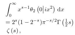
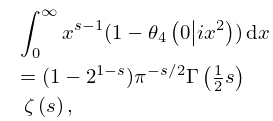
15: 20.10 Integrals

… ►

§20.10(i) Mellin Transforms with respect to the Lattice Parameter

►

20.10.1 $${\int }_0^{\mathrm{\infty }}{x}^{s-1}{\theta }_2\left(0\right|\mathrm{i}{x}^2)dx=2^s(1-2^{-s}){\pi }^{-s/2}\mathrm{\Gamma }\left(\frac{1}{2}s\right)\zeta \left(s\right),$$ $\mathrm{\Re }s>1$,

ⓘ

Symbols:

$\mathrm{\Gamma }\left(z\right)$: gamma function, ${\theta }_j\left(z\right|\tau )$: theta function, $\zeta \left(s\right)$: Riemann zeta function, $\pi$: the ratio of the circumference of a circle to its diameter, $dx$: differential of $x$ , $\mathrm{i}$: imaginary unit, $\int$: integral and $\mathrm{\Re }$: real part

Keywords:

Mellin transform

Referenced by:

§20.10(i), Erratum (V1.1.5) for §20.10(i)

Permalink:

http://dlmf.nist.gov/20.10.E1

Encodings:

pMML, png, TeX

Modification (effective with 1.1.5):

Originally the constraint was $\mathrm{\Re }s>2$. This can be relaxed to $\mathrm{\Re }s>1$ because ${\theta }_2\left(0\right|\mathrm{i}{x}^2)=x^{-1}{\theta }_4\left(0\right|\mathrm{i}{x}^{-2})\sim x^{-1}$ as $x\to 0+$, which follows from (20.7.31) and (20.4.5).

See also:

Annotations for §20.10(i), §20.10 and Ch.20

►

20.10.2 $${\int }_0^{\mathrm{\infty }}{x}^{s-1}({\theta }_3\left(0\right|\mathrm{i}{x}^2)-1)dx={\pi }^{-s/2}\mathrm{\Gamma }\left(\frac{1}{2}s\right)\zeta \left(s\right),$$ $\mathrm{\Re }s>1$,

ⓘ

Symbols:

$\mathrm{\Gamma }\left(z\right)$: gamma function, ${\theta }_j\left(z\right|\tau )$: theta function, $\zeta \left(s\right)$: Riemann zeta function, $\pi$: the ratio of the circumference of a circle to its diameter, $dx$: differential of $x$ , $\mathrm{i}$: imaginary unit, $\int$: integral and $\mathrm{\Re }$: real part

Keywords:

Mellin transform

Referenced by:

§20.10(i), Erratum (V1.1.5) for §20.10(i)

Permalink:

http://dlmf.nist.gov/20.10.E2

Encodings:

pMML, png, TeX

Modification (effective with 1.1.5):

Originally the constraint was $\mathrm{\Re }s>2$. This can be relaxed to $\mathrm{\Re }s>1$ because ${\theta }_3\left(0\right|\mathrm{i}{x}^2)=x^{-1}{\theta }_3\left(0\right|\mathrm{i}{x}^{-2})\sim x^{-1}$ as $x\to 0+$, which follows from (20.7.32) and (20.4.4).

See also:

Annotations for §20.10(i), §20.10 and Ch.20

►

20.10.3 $${\int }_0^{\mathrm{\infty }}{x}^{s-1}(1-{\theta }_4\left(0\right|\mathrm{i}{x}^2))dx=(1-2^{1-s}){\pi }^{-s/2}\mathrm{\Gamma }\left(\frac{1}{2}s\right)\zeta \left(s\right),$$ $\mathrm{\Re }s>0$.

ⓘ

Symbols:

$\mathrm{\Gamma }\left(z\right)$: gamma function, ${\theta }_j\left(z\right|\tau )$: theta function, $\zeta \left(s\right)$: Riemann zeta function, $\pi$: the ratio of the circumference of a circle to its diameter, $dx$: differential of $x$ , $\mathrm{i}$: imaginary unit, $\int$: integral and $\mathrm{\Re }$: real part

Keywords:

Mellin transform

Referenced by:

§20.10(i), Erratum (V1.1.5) for §20.10(i)

Permalink:

http://dlmf.nist.gov/20.10.E3

Encodings:

pMML, png, TeX

Modification (effective with 1.1.5):

Originally the constraint was $\mathrm{\Re }s>2$. This can be relaxed to $\mathrm{\Re }s>0$ because $1-{\theta }_4\left(0\right|\mathrm{i}{x}^2)=1-x^{-1}{\theta }_2\left(0\right|\mathrm{i}{x}^{-2})\sim 1$ as $x\to 0+$, which follows from (20.7.33) and (20.4.3).

See also:

Annotations for §20.10(i), §20.10 and Ch.20

… ►

§20.10(ii) Laplace Transforms with respect to the Lattice Parameter

…

16: Bibliography O

… ►

Tables of Lebedev, Mehler and Generalized Mehler Transforms. Mathematical Note Technical Report 246, Boeing Scientific Research Lab, Seattle.

ⓘ

Referenced by:

§1.14(viii).

Encodings:

BibTeX

►

Tables of Fourier Transforms and Fourier Transforms of Distributions. Springer-Verlag, Berlin.

ⓘ

External Links:

ISBN 3-540-50630-6; 0-387-50630-6, MathReview, ZentralBlatt

Referenced by:

§1.14(viii), §10.22(vi), §10.43(vi), §11.10(x), §11.7(v), §11.9(iv), §12.12, §13.10(iv), §13.23(ii), §18.17(ix), §6.14(iii), §7.14(iii).

Encodings:

BibTeX

… ►

Tables of Bessel Transforms. Springer-Verlag, Berlin-New York.

ⓘ

Notes:

Table errata: Math. Comp. v. 65 (1996), no. 215, p. 1386.

External Links:

ISBN 0-387-05997-0, MathReview, ZentralBlatt

Referenced by:

§1.14(viii), §10.22(v), §10.43(v), §10.43(vi), §11.10(x), §11.5(iii), §11.7(v), §11.9(iv), §13.10(v), §13.23(iii), §15.14, §18.17(ix), §8.14, §8.6(iii).

Encodings:

BibTeX

… ►

Tables of Mellin Transforms. Springer-Verlag, Berlin-New York.

ⓘ

External Links:

ISBN 0-387-06942-9, MathReview, ZentralBlatt

Referenced by:

§1.14(viii), §10.22(vi), §10.43(vi), §11.10(x), §11.5(iii), §11.7(v), §11.9(iv), §12.12, §12.5(iv), §13.10(iii), §13.23(i), §14.17(vi), §15.14, §18.17(ix), §20.10(i), §5.13, §6.14(iii), §6.7(iv), §7.14(iii), §7.7(iii).

Encodings:

BibTeX

… ►

An error analysis of the modified Clenshaw method for evaluating Chebyshev and Fourier series. J. Inst. Math. Appl. 20 (3), pp. 379–391.

ⓘ

External Links:

Document, MathReview (David L. Elliott), ZentralBlatt

Referenced by:

§3.11(ii).

Encodings:

BibTeX

…

17: 3.4 Differentiation

… ►If $f^{(n+2)}(x)$ is continuous on the interval $I$ defined in §3.3(i), then the remainder in (3.4.1) is given by … ►where $C$ is a simple closed contour described in the positive rotational sense such that $C$ and its interior lie in the domain of analyticity of $f$, and $x_0$ is interior to $C$. Taking $C$ to be a circle of radius $r$ centered at $x_0$, we obtain … ►

First-Order

… ►For additional formulas involving values of ${\nabla }^{2}u$ and ${\nabla }^{4}u$ on square, triangular, and cubic grids, see Collatz (1960, Table VI, pp. 542–546). …

18: 33.24 Tables

… ►

Abramowitz and Stegun (1964, Chapter 14) tabulates $F_0(\eta ,\rho )$, $G_0(\eta ,\rho )$, $F_0^{\prime }(\eta ,\rho )$, and $G_0^{\prime }(\eta ,\rho )$ for $\eta =0.5(.5)20$ and $\rho =1(1)20$, 5S; $C_0\left(\eta \right)$ for $\eta =0(.05)3$, 6S.

►

Curtis (1964a) tabulates $P_{\mathrm{\ell }}(ϵ,r)$, $Q_{\mathrm{\ell }}(ϵ,r)$ (§33.1), and related functions for $\mathrm{\ell }=0,1,2$ and $ϵ=-2(.2)2$, with $x=0(.1)4$ for and $x=0(.1)10$ for $ϵ\ge 0$; 6D.

…

19: Errata

… ►

There have been extensive changes in the notation used for the integral transforms defined in §1.14. These changes are applied throughout the DLMF. The following table summarizes the changes.

Transform	New	Abbreviated	Old
	Notation	Notation	Notation
Fourier	$ℱ\left(f\right)\left(x\right)$	$ℱf\left(x\right)$
Fourier Cosine	${ℱ}_c\left(f\right)\left(x\right)$	${ℱ}_{c}f\left(x\right)$
Fourier Sine	${ℱ}_s\left(f\right)\left(x\right)$	${ℱ}_{s}f\left(x\right)$
Laplace	$ℒ\left(f\right)\left(s\right)$	$ℒf\left(s\right)$	$ℒ(f(t);s)$
Mellin	$ℳ\left(f\right)\left(s\right)$	$ℳf\left(s\right)$	$ℳ(f;s)$
Hilbert	$\mathscr{H}\left(f\right)\left(s\right)$	$\mathscr{H}f\left(s\right)$	$\mathscr{H}(f;s)$
Stieltjes	$𝒮\left(f\right)\left(s\right)$	$𝒮f\left(s\right)$	$𝒮(f;s)$

Previously, for the Fourier, Fourier cosine and Fourier sine transforms, either temporary local notations were used or the Fourier integrals were written out explicitly.

… ►

An entire new Subsection 1.16(viii) Fourier Transforms of Special Distributions, was contributed by Roderick Wong.

… ►

The title was changed from Transformations of Higher ${}_r{}^{}\varphi _r^{}$ Functions to Further Transformations of ${}_{r+1}{}^{}\varphi _r^{}$ Functions.

… ►

Several new equations have been added. See (8.17.24), (20.7.34), §20.11(v), (26.12.27), (36.2.28), and (36.2.29).

… ►

Bibliographic citations were added in §§1.13(v), 10.14, 10.21(ii), 18.15(v), 18.32, 30.16(iii), 32.13(ii), and as general references in Chapters 19, 20, 22, and 23.

…

20: Staff

… ►

William P. Reinhardt, University of Washington, Chaps. 20, 22, 23

… ►

Peter L. Walker, American University of Sharjah, Chaps. 20, 22, 23

►

Gerhard Wolf, University of Duisberg-Essen, Chap. 28

… ►

William P. Reinhardt, University of Washington, for Chaps. 20, 22, 23

… ►

Peter L. Walker, American University of Sharjah, for Chaps. 20, 22, 23

…