§18.15 Asymptotic Approximations
Contents
- §18.15(i) Jacobi
- §18.15(ii) Ultraspherical
- §18.15(iii) Legendre
- §18.15(iv) Laguerre
- §18.15(v) Hermite
- §18.15(vi) Other Approximations
§18.15(i) Jacobi
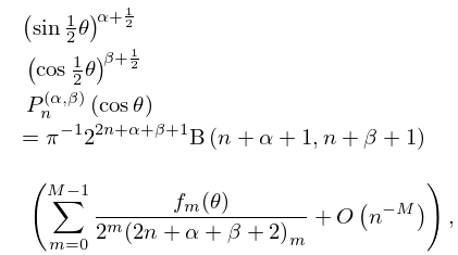
With the exception of the penultimate paragraph, we assume throughout this subsection that , , and () are all fixed.
| 18.15.1 | |||
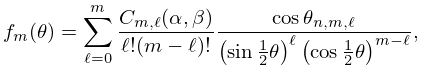
as , uniformly with respect to . Here, and elsewhere in §18.15, is an arbitrary small positive constant. Also, is the beta function (§5.12) and
| 18.15.2 | |||
where
| 18.15.3 | |||
and
| 18.15.4 | |||
When , the error term in (18.15.1) is less than twice the first neglected term in absolute value, in which one has to take . See Hahn (1980), where corresponding results are given when is replaced by a complex variable that is bounded away from the orthogonality interval .
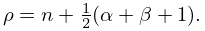
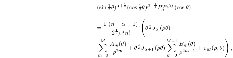
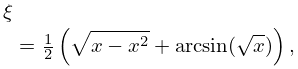
Next, let
| 18.15.5 | |||
Then as ,
| 18.15.6 | |||
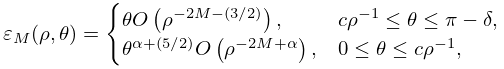
where is the Bessel function (§10.2(ii)), and
| 18.15.7 | |||
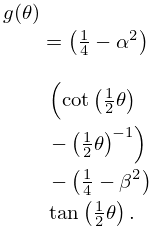
with denoting an arbitrary positive constant. Also,
| 18.15.8 | ||||
where
| 18.15.9 | |||
For higher coefficients see Baratella and Gatteschi (1988), and for another estimate of the error term in a related expansion see Wong and Zhao (2003). For large , fixed , and , Dunster (1999) gives asymptotic expansions of that are uniform in unbounded complex -domains containing . These expansions are in terms of Whittaker functions (§13.14). This reference also supplies asymptotic expansions of for large , fixed , and . The latter expansions are in terms of Bessel functions, and are uniform in complex -domains not containing neighborhoods of 1. For a complementary result, see Wong and Zhao (2004). By using the symmetry property given in the second row of Table 18.6.1, the roles of and can be interchanged.
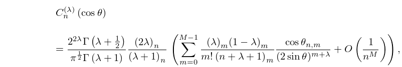
§18.15(ii) Ultraspherical
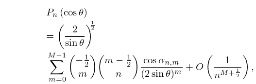
§18.15(iii) Legendre
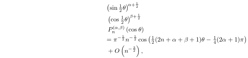
For fixed ,
| 18.15.12 | |||
as , uniformly with respect to , where
| 18.15.13 | |||
Also, when , the right-hand side of (18.15.12) with converges; paradoxically, however, the sum is and not as stated erroneously in Szegő (1975, §8.4(3)).
For these results and further information see Olver (1997b, pp. 311–313). Another expansion follows from (18.15.10) by taking ; see Szegő (1975, Theorem 8.21.5).
For asymptotic expansions of and that are uniformly valid when and see §14.15(iii) with and . These expansions are in terms of Bessel functions and modified Bessel functions, respectively.
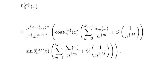
§18.15(iv) Laguerre
In Terms of Elementary Functions
For fixed , and fixed ,
| 18.15.14 | |||
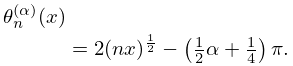
as , uniformly on compact -intervals in , where
| 18.15.15 | |||
The leading coefficients are given by
| 18.15.16 | ||||
See also Deaño et al. (2013).
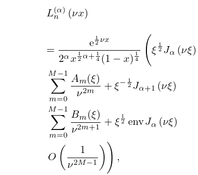
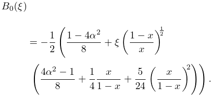
In Terms of Bessel Functions
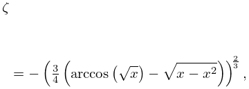
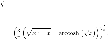
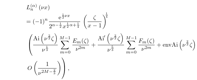
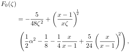
In Terms of Airy Functions
§18.15(v) Hermite
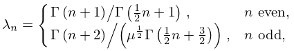
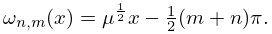
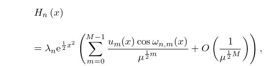
Define
| 18.15.24 | |||
| 18.15.25 | |||
and
| 18.15.26 | |||
Then for fixed ,
| 18.15.27 | |||
as , uniformly on compact -intervals on . The coefficients are polynomials in , and , .
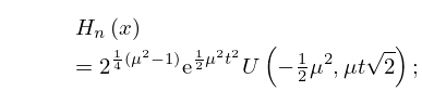
For more powerful asymptotic expansions as in terms of elementary functions that apply uniformly when , , or , where and is again an arbitrary small positive constant, see §§12.10(i)–12.10(iv) and 12.10(vi). And for asymptotic expansions as in terms of Airy functions that apply uniformly when or , see §§12.10(vii) and 12.10(viii). With the expansions in Chapter 12 are for the parabolic cylinder function , which is related to the Hermite polynomials via
| 18.15.28 | |||
compare (18.11.3).
For an error bound for the first term in the Airy-function expansions see Olver (1997b, p. 403).
See also Geronimo et al. (2004).
§18.15(vi) Other Approximations
The asymptotic behavior of the classical OP’s as with the degree and parameters fixed is evident from their explicit polynomial forms; see, for example, (18.2.7) and the last two columns of Table 18.3.1.
For asymptotic approximations of Jacobi, ultraspherical, and Laguerre polynomials in terms of Hermite polynomials, see López and Temme (1999a). These approximations apply when the parameters are large, namely and (subject to restrictions) in the case of Jacobi polynomials, in the case of ultraspherical polynomials, and in the case of Laguerre polynomials. See also Dunster (1999), Atia et al. (2014) and Temme (2015, Chapter 32).
