Euler%20totient

SearchAdvancedHelp

(0.002 seconds)

21—30 of 452 matching pages

21: 25.12 Polylogarithms

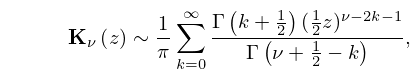
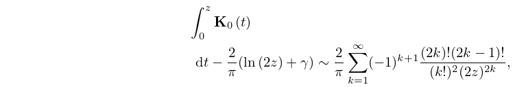
… ►The notation ${\mathrm{Li}}_2\left(z\right)$ was introduced in Lewin (1981) for a function discussed in Euler (1768) and called the dilogarithm in Hill (1828): … ►

►►

Figure 25.12.1: Dilogarithm function ${\mathrm{Li}}_2\left(x\right)$, Magnify

►

►

►

Figure 25.12.2: Absolute value of the dilogarithm function $\left|{\mathrm{Li}}_2\left(x+\mathrm{i}y\right)\right|$, $-20\le x\le 20$, $-20\le y\le 20$. … Magnify 3D Help

… ►

25.12.11 $${\mathrm{Li}}_s\left(z\right)\equiv \frac{z}{\mathrm{\Gamma }\left(s\right)}{\int }_0^{\mathrm{\infty }}\frac{x^{s-1}}{{\mathrm{e}}^x-z}dx,$$

ⓘ

Symbols:

$\mathrm{\Gamma }\left(z\right)$: gamma function, $dx$: differential of $x$ , $\equiv$: equals by definition, $\mathrm{e}$: base of natural logarithm, $\int$: integral, ${\mathrm{Li}}_s\left(z\right)$: polylogarithm, $x$: real variable, $s$: complex variable and $z$: complex variable

Keywords:

improper integral, integral representation

Source:

Lewin (1981, (7.188), p. 236)

Referenced by:

(25.12.16), §25.12(ii)

Permalink:

http://dlmf.nist.gov/25.12.E11

Encodings:

pMML, png, TeX

See also:

Annotations for §25.12(ii), §25.12(ii), §25.12 and Ch.25

… ►Sometimes the factor $1/\mathrm{\Gamma }\left(s+1\right)$ is omitted. …

22: 5.11 Asymptotic Expansions

… ►The scaled gamma function ${\mathrm{\Gamma }}^{\ast }\left(z\right)$ is defined in (5.11.3) and its main property is ${\mathrm{\Gamma }}^{\ast }\left(z\right)\sim 1$ as $z\to \mathrm{\infty }$ in the sector $|\mathrm{ph}z|\le \pi -\delta$. Wrench (1968) gives exact values of $g_k$ up to $g_{20}$. … ►

5.11.12 $$\frac{\mathrm{\Gamma }\left(z+a\right)}{\mathrm{\Gamma }\left(z+b\right)}\sim z^{a-b},$$

ⓘ

Symbols:

$\mathrm{\Gamma }\left(z\right)$: gamma function, $\sim$: asymptotic equality, $z$: complex variable, $a$: real or complex variable and $b$: real or complex variable

Referenced by:

§5.11(i)

Permalink:

http://dlmf.nist.gov/5.11.E12

Encodings:

pMML, png, TeX

See also:

Annotations for §5.11(iii), §5.11 and Ch.5

►

5.11.13 $$\frac{\mathrm{\Gamma }\left(z+a\right)}{\mathrm{\Gamma }\left(z+b\right)}\sim z^{a-b}\sum _{k=0}^{\mathrm{\infty }}\frac{G_k(a,b)}{z^k},$$

ⓘ

Symbols:

$\mathrm{\Gamma }\left(z\right)$: gamma function, $\sim$: Poincaré asymptotic expansion, $k$: nonnegative integer, $z$: complex variable, $a$: real or complex variable, $b$: real or complex variable and $G_k(a,b)$: coefficients

A&S Ref:

6.1.47

Permalink:

http://dlmf.nist.gov/5.11.E13

Encodings:

pMML, png, TeX

See also:

Annotations for §5.11(iii), §5.11 and Ch.5

… ►

5.11.19 $$\frac{\mathrm{\Gamma }\left(z+a\right)\mathrm{\Gamma }\left(z+b\right)}{\mathrm{\Gamma }\left(z+c\right)}\sim \sum _{k=0}^{\mathrm{\infty }}{(-1)}^k\frac{{\left(c-a\right)}_k{\left(c-b\right)}_k}{k!}\mathrm{\Gamma }\left(a+b-c+z-k\right).$$

ⓘ

Symbols:

$\mathrm{\Gamma }\left(z\right)$: gamma function, ${\left(a\right)}_n$: Pochhammer’s symbol (or shifted factorial), $\sim$: Poincaré asymptotic expansion, $!$: factorial (as in $n!$), $k$: nonnegative integer, $z$: complex variable, $a$: real or complex variable and $b$: real or complex variable

Referenced by:

§5.11(i), §5.11(iii)

Permalink:

http://dlmf.nist.gov/5.11.E19

Encodings:

pMML, png, TeX

See also:

Annotations for §5.11(iii), §5.11 and Ch.5

…

23: 24.18 Physical Applications

§24.18 Physical Applications

►Bernoulli polynomials appear in statistical physics (Ordóñez and Driebe (1996)), in discussions of Casimir forces (Li et al. (1991)), and in a study of quark-gluon plasma (Meisinger et al. (2002)). ►Euler polynomials also appear in statistical physics as well as in semi-classical approximations to quantum probability distributions (Ballentine and McRae (1998)).

24: 25.20 Approximations

… ►

Cody et al. (1971) gives rational approximations for $\zeta \left(s\right)$ in the form of quotients of polynomials or quotients of Chebyshev series. The ranges covered are $0.5\le s\le 5$, $5\le s\le 11$, $11\le s\le 25$, $25\le s\le 55$. Precision is varied, with a maximum of 20S.

… ►

Antia (1993) gives minimax rational approximations for $\mathrm{\Gamma }\left(s+1\right)F_s(x)$, where $F_s(x)$ is the Fermi–Dirac integral (25.12.14), for the intervals and , with $s=-\frac{1}{2},\frac{1}{2},\frac{3}{2},\frac{5}{2}$. For each $s$ there are three sets of approximations, with relative maximum errors ${10}^{-4},{10}^{-8},{10}^{-12}$.

25: 8.17 Incomplete Beta Functions

… ►

8.17.2 $$I_x(a,b)={\mathrm{B}}_x(a,b)/\mathrm{B}(a,b),$$

ⓘ

Defines:

$I_x(a,b)$: incomplete beta function

Symbols:

$\mathrm{B}(a,b)$: beta function, ${\mathrm{B}}_x(a,b)$: incomplete beta function, $a$: parameter, $b$: parameter and $x$: variable

A&S Ref:

6.6.2

Permalink:

http://dlmf.nist.gov/8.17.E2

Encodings:

pMML, png, TeX

See also:

Annotations for §8.17(i), §8.17 and Ch.8

►where, as in §5.12, $\mathrm{B}(a,b)$ denotes the beta function: ►

8.17.3 $$\mathrm{B}(a,b)=\frac{\mathrm{\Gamma }\left(a\right)\mathrm{\Gamma }\left(b\right)}{\mathrm{\Gamma }\left(a+b\right)}.$$

ⓘ

Symbols:

$\mathrm{B}(a,b)$: beta function, $\mathrm{\Gamma }\left(z\right)$: gamma function, $a$: parameter and $b$: parameter

Permalink:

http://dlmf.nist.gov/8.17.E3

Encodings:

pMML, png, TeX

See also:

Annotations for §8.17(i), §8.17 and Ch.8

… ►

8.17.20 $$I_x(a,b)=I_x(a+1,b)+\frac{x^a{(x^{\prime })}^b}{a\mathrm{B}(a,b)},$$

ⓘ

Symbols:

$\mathrm{B}(a,b)$: beta function, $I_x(a,b)$: incomplete beta function, $a$: parameter, $b$: parameter, $x$: variable and $x^{\prime }$

Permalink:

http://dlmf.nist.gov/8.17.E20

Encodings:

pMML, png, TeX

See also:

Annotations for §8.17(iv), §8.17 and Ch.8

►

8.17.21 $$I_x(a,b)=I_x(a,b+1)-\frac{x^a{(x^{\prime })}^b}{b\mathrm{B}(a,b)}.$$

ⓘ

Symbols:

$\mathrm{B}(a,b)$: beta function, $I_x(a,b)$: incomplete beta function, $a$: parameter, $b$: parameter, $x$: variable and $x^{\prime }$

Permalink:

http://dlmf.nist.gov/8.17.E21

Encodings:

pMML, png, TeX

See also:

Annotations for §8.17(iv), §8.17 and Ch.8

…

26: 11.6 Asymptotic Expansions

… ►

11.6.1 $${𝐊}_{\nu }\left(z\right)\sim \frac{1}{\pi }\sum _{k=0}^{\mathrm{\infty }}\frac{\mathrm{\Gamma }\left(k+\frac{1}{2}\right){(\frac{1}{2}z)}^{\nu -2k-1}}{\mathrm{\Gamma }\left(\nu +\frac{1}{2}-k\right)},$$ $|\mathrm{ph}z|\le \pi -\delta$,

ⓘ

Symbols:

$\mathrm{\Gamma }\left(z\right)$: gamma function, ${𝐊}_{\nu }\left(z\right)$: Struve function, $\sim$: Poincaré asymptotic expansion, $\pi$: the ratio of the circumference of a circle to its diameter, $\mathrm{ph}$: phase, $z$: complex variable, $\nu$: real or complex order, $k$: nonnegative integer and $\delta$: arbitrary small positive constant

A&S Ref:

12.1.29

Referenced by:

§11.6(i), §11.6(i), §11.6(i), §11.6(i)

Permalink:

http://dlmf.nist.gov/11.6.E1

Encodings:

pMML, png, TeX

See also:

Annotations for §11.6(i), §11.6 and Ch.11

… ►

11.6.2 $${𝐌}_{\nu }\left(z\right)\sim \frac{1}{\pi }\sum _{k=0}^{\mathrm{\infty }}{(-1)}^{k+1}\frac{\mathrm{\Gamma }\left(k+\frac{1}{2}\right){(\frac{1}{2}z)}^{\nu -2k-1}}{\mathrm{\Gamma }\left(\nu +\frac{1}{2}-k\right)},$$ $|\mathrm{ph}z|\le \frac{1}{2}\pi -\delta$.

ⓘ

Symbols:

$\mathrm{\Gamma }\left(z\right)$: gamma function, ${𝐌}_{\nu }\left(z\right)$: modified Struve function, $\sim$: Poincaré asymptotic expansion, $\pi$: the ratio of the circumference of a circle to its diameter, $\mathrm{ph}$: phase, $z$: complex variable, $\nu$: real or complex order, $k$: nonnegative integer and $\delta$: arbitrary small positive constant

A&S Ref:

12.2.6

Referenced by:

§11.6(i), §11.6(i), §11.6(i)

Permalink:

http://dlmf.nist.gov/11.6.E2

Encodings:

pMML, png, TeX

See also:

Annotations for §11.6(i), §11.6 and Ch.11

… ►

11.6.3 $${\int }_0^z{𝐊}_0\left(t\right)dt-\frac{2}{\pi }(\ln \left(2z\right)+\gamma )\sim \frac{2}{\pi }\sum _{k=1}^{\mathrm{\infty }}{(-1)}^{k+1}\frac{(2k)!(2k-1)!}{{(k!)}^2{(2z)}^{2k}},$$ $|\mathrm{ph}z|\le \pi -\delta$,

ⓘ

Symbols:

$\gamma$: Euler’s constant, ${𝐊}_{\nu }\left(z\right)$: Struve function, $\sim$: Poincaré asymptotic expansion, $\pi$: the ratio of the circumference of a circle to its diameter, $dx$: differential of $x$ , $!$: factorial (as in $n!$), $\int$: integral, $\ln z$: principal branch of logarithm function, $\mathrm{ph}$: phase, $z$: complex variable, $k$: nonnegative integer and $\delta$: arbitrary small positive constant

A&S Ref:

12.1.32

Referenced by:

§11.6(i)

Permalink:

http://dlmf.nist.gov/11.6.E3

Encodings:

pMML, png, TeX

See also:

Annotations for §11.6(i), §11.6 and Ch.11

… ►where $\gamma$ is Euler’s constant (§5.2(ii)). … ►

$c_3(\lambda )=20{\lambda }^{-6}-4{\lambda }^{-4},$

…

27: 24.3 Graphs

… ►

►►

Figure 24.3.2: Euler polynomials $E_n\left(x\right)$, $n=2,3,\mathrm{\dots },6$. Magnify

28: 25.6 Integer Arguments

… ►

§25.6(i) Function Values

… ►

25.6.3 $$\zeta \left(-n\right)=-\frac{B_{n+1}}{n+1},$$ $n=1,2,3,\mathrm{\dots }$.

ⓘ

Symbols:

$B_n$: Bernoulli numbers, $\zeta \left(s\right)$: Riemann zeta function and $n$: nonnegative integer

Source:

Apostol (1976, (20), p. 266); with $n\ne 0$

A&S Ref:

23.2.15 (in slightly different form)

Permalink:

http://dlmf.nist.gov/25.6.E3

Encodings:

pMML, png, TeX

See also:

Annotations for §25.6(i), §25.6 and Ch.25

… ►

25.6.12 $${\zeta }^{\prime \prime }\left(0\right)=-\frac{1}{2}{(\ln \left(2\pi \right))}^2+\frac{1}{2}{\gamma }^2-\frac{1}{24}{\pi }^2+{\gamma }_1,$$

ⓘ

Symbols:

$\gamma$: Euler’s constant, $\zeta \left(s\right)$: Riemann zeta function, ${\gamma }_n$: Stieltjes constants, $\pi$: the ratio of the circumference of a circle to its diameter and $\ln z$: principal branch of logarithm function

Source:

Apostol (1985a, pp. 226, 227, 229)

Referenced by:

Erratum (V1.0.23) for Subsection 25.2(ii) Other Infinite Series

Permalink:

http://dlmf.nist.gov/25.6.E12

Encodings:

pMML, png, TeX

See also:

Annotations for §25.6(ii), §25.6 and Ch.25

►where ${\gamma }_1$ is given by (25.2.5). … ►

25.6.13 $${(-1)}^k{\zeta }^{(k)}\left(-2n\right)=\frac{2{(-1)}^n}{{(2\pi )}^{2n+1}}\sum _{m=0}^k\sum _{r=0}^m\left(\genfrac{}{}{0.0pt}{}{k}{m}\right)\left(\genfrac{}{}{0.0pt}{}{m}{r}\right)\mathrm{\Im }\left(c^{k-m}\right){\mathrm{\Gamma }}^{(r)}\left(2n+1\right){\zeta }^{(m-r)}\left(2n+1\right),$$

ⓘ

Symbols:

$\mathrm{\Gamma }\left(z\right)$: gamma function, $\zeta \left(s\right)$: Riemann zeta function, $\left(\genfrac{}{}{0.0pt}{}{m}{n}\right)$: binomial coefficient, $\pi$: the ratio of the circumference of a circle to its diameter, $\mathrm{\Im }$: imaginary part, $k$: nonnegative integer, $m$: nonnegative integer, $n$: nonnegative integer and $c$

Source:

Apostol (1985a, p. 225)

Permalink:

http://dlmf.nist.gov/25.6.E13

Encodings:

pMML, png, TeX

See also:

Annotations for §25.6(ii), §25.6 and Ch.25

…

29: 25.5 Integral Representations

… ►

25.5.1 $$\zeta \left(s\right)=\frac{1}{\mathrm{\Gamma }\left(s\right)}{\int }_0^{\mathrm{\infty }}\frac{x^{s-1}}{{\mathrm{e}}^x-1}dx,$$ $\mathrm{\Re }s>1$.

ⓘ

Symbols:

$\mathrm{\Gamma }\left(z\right)$: gamma function, $\zeta \left(s\right)$: Riemann zeta function, $dx$: differential of $x$ , $\mathrm{e}$: base of natural logarithm, $\int$: integral, $\mathrm{\Re }$: real part, $x$: real variable and $s$: complex variable

Keywords:

improper integral, integral representation

Source:

Erdélyi et al. (1953a, (1.12.4), p. 32)

A&S Ref:

23.2.7

Referenced by:

§25.12(ii), (25.5.2), (25.5.6)

Permalink:

http://dlmf.nist.gov/25.5.E1

Encodings:

pMML, png, TeX

See also:

Annotations for §25.5(i), §25.5 and Ch.25

… ►

25.5.13 $$\zeta \left(s\right)=\frac{{\pi }^{s/2}}{s(s-1)\mathrm{\Gamma }\left(\frac{1}{2}s\right)}+\frac{{\pi }^{s/2}}{\mathrm{\Gamma }\left(\frac{1}{2}s\right)}{\int }_1^{\mathrm{\infty }}\left(x^{s/2}+x^{(1-s)/2}\right)\frac{\omega (x)}{x}dx,$$ $s\ne 1$,

ⓘ

Symbols:

$\mathrm{\Gamma }\left(z\right)$: gamma function, $\zeta \left(s\right)$: Riemann zeta function, $\pi$: the ratio of the circumference of a circle to its diameter, $dx$: differential of $x$ , $\int$: integral, $x$: real variable and $s$: complex variable

Keywords:

improper integral, integral representation

Source:

Titchmarsh (1986b, p. 22)

Permalink:

http://dlmf.nist.gov/25.5.E13

Encodings:

pMML, png, TeX

See also:

Annotations for §25.5(ii), §25.5 and Ch.25

… ►In (25.5.15)–(25.5.19), , $\psi \left(x\right)$ is the digamma function, and $\gamma$ is Euler’s constant (§5.2). … ►

25.5.17 $$\zeta \left(1+s\right)=\frac{\sin \left(\pi s\right)}{\pi }{\int }_0^{\mathrm{\infty }}\left(\gamma +\psi \left(1+x\right)\right)x^{-s-1}dx,$$

ⓘ

Symbols:

$\gamma$: Euler’s constant, $\zeta \left(s\right)$: Riemann zeta function, $\pi$: the ratio of the circumference of a circle to its diameter, $dx$: differential of $x$ , $\psi \left(z\right)$: psi (or digamma) function, $\int$: integral, $\sin z$: sine function, $x$: real variable and $s$: complex variable

Keywords:

improper integral, integral representation

Source:

de Bruijn (1937, (22), p. 177)

Permalink:

http://dlmf.nist.gov/25.5.E17

Encodings:

pMML, png, TeX

See also:

Annotations for §25.5(ii), §25.5 and Ch.25

… ►

25.5.19 $$\zeta \left(m+s\right)={(-1)}^{m-1}\frac{\mathrm{\Gamma }\left(s\right)\sin \left(\pi s\right)}{\pi \mathrm{\Gamma }\left(m+s\right)}{\int }_0^{\mathrm{\infty }}{\psi }^{(m)}\left(1+x\right)x^{-s}dx,$$ $m=1,2,3,\mathrm{\dots }$.

ⓘ

Symbols:

$\mathrm{\Gamma }\left(z\right)$: gamma function, $\zeta \left(s\right)$: Riemann zeta function, $\pi$: the ratio of the circumference of a circle to its diameter, $dx$: differential of $x$ , $\psi \left(z\right)$: psi (or digamma) function, $\int$: integral, $\sin z$: sine function, $m$: nonnegative integer, $x$: real variable and $s$: complex variable

Keywords:

improper integral, integral representation

Source:

de Bruijn (1937, p. 178)

Referenced by:

§25.5(ii)

Permalink:

http://dlmf.nist.gov/25.5.E19

Encodings:

pMML, png, TeX

See also:

Annotations for §25.5(ii), §25.5 and Ch.25

…

30: Errata

… ►

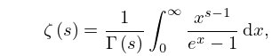
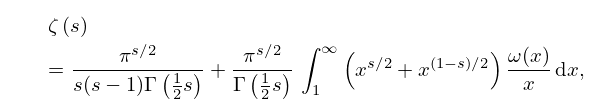
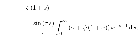
It is now mentioned that (25.2.5), defines the Stieltjes constants ${\gamma }_n$. Consequently, ${\gamma }_n$ in (25.2.4), (25.6.12) are now identified as the Stieltjes constants.

… ►

27.12.8 $$\frac{\mathrm{li}\left(x\right)}{\varphi \left(m\right)}+O\left(x\exp \left(-\lambda (\alpha ){(\ln x)}^{1/2}\right)\right),$$ $m\le {(\ln x)}^{\alpha }$, $\alpha >0$

Originally the first term was given incorrectly by $\frac{x}{\varphi \left(m\right)}$.

Reported 2017-12-04 by Gergő Nemes.

… ►

Several new equations have been added. See (8.17.24), (20.7.34), §20.11(v), (26.12.27), (36.2.28), and (36.2.29).

… ►

17.13.3 $${\int }_0^{\mathrm{\infty }}{t}^{\alpha -1}\frac{{(-t{q}^{\alpha +\beta };q)}_{\mathrm{\infty }}}{{(-t;q)}_{\mathrm{\infty }}}dt=\frac{\mathrm{\Gamma }\left(\alpha \right)\mathrm{\Gamma }\left(1-\alpha \right){\mathrm{\Gamma }}_q\left(\beta \right)}{{\mathrm{\Gamma }}_q\left(1-\alpha \right){\mathrm{\Gamma }}_q\left(\alpha +\beta \right)}$$

Originally the differential was identified incorrectly as $d_{q}t$; the correct differential is $dt$.

Reported 2011-04-08.

… ►

Bibliographic citations were added in §§1.13(v), 10.14, 10.21(ii), 18.15(v), 18.32, 30.16(iii), 32.13(ii), and as general references in Chapters 19, 20, 22, and 23.

…