Euler%20sums
(0.001 seconds)
11—19 of 19 matching pages
11: 32.8 Rational Solutions
…
►In the general case assume , so that as in §32.2(ii) we may set and .
…
►
(a)
…
►
(c)
►
(d)
►
(e)
…
and , where , is odd, and when .
, , and , with even.
, , and , with even.
, , and .
12: 12.10 Uniform Asymptotic Expansions for Large Parameter
…
►
…
12.10.14
…
►and the coefficients are defined by
►
12.10.16
…
►where and are as in §12.10(ii).
…
►
13: 2.11 Remainder Terms; Stokes Phenomenon
…
►The transformations in §3.9 for summing slowly convergent series can also be very effective when applied to divergent asymptotic series.
…
►Multiplying these differences by and summing, we obtain
…Subtraction of this result from the sum of the first 5 terms in (2.11.25) yields 0.
…
…
►For example, using double precision is found to agree with (2.11.31) to 13D.
…
14: Bibliography B
…
►
Pionic atoms.
Annual Review of Nuclear and Particle Science 20, pp. 467–508.
…
►
A program for computing the Riemann zeta function for complex argument.
Comput. Phys. Comm. 20 (3), pp. 441–445.
…
►
A new method for investigating Euler sums.
Ramanujan J. 4 (4), pp. 397–419.
…
►
Coulomb functions (negative energies).
Comput. Phys. Comm. 20 (3), pp. 447–458.
…
►
Some solutions of the problem of forced convection.
Philos. Mag. Series 7 20, pp. 322–343.
…
15: Errata
…
►
Additions
…
►
Equation (8.18.3)
…
►
Equation (5.17.5)
…
►
Chapters 8, 20, 36
…
►
References
…
8.18.3
The range of was extended to include . Previously this equation appeared without the order estimate as .
Reported 2016-08-30 by Xinrong Ma.
5.17.5
Originally the term was incorrectly stated as .
Reported 2013-08-01 by Gergő Nemes and subsequently by Nick Jones on December 11, 2013.
16: Bibliography L
…
►
Algorithm 917: complex double-precision evaluation of the Wright function.
ACM Trans. Math. Software 38 (3), pp. Art. 20, 17.
…
►
An asymptotic estimate for the Bernoulli and Euler numbers.
Canad. Math. Bull. 20 (1), pp. 109–111.
…
►
Hermite polynomials in asymptotic representations of generalized Bernoulli, Euler, Bessel, and Buchholz polynomials.
J. Math. Anal. Appl. 239 (2), pp. 457–477.
►
Uniform approximations of Bernoulli and Euler polynomials in terms of hyperbolic functions.
Stud. Appl. Math. 103 (3), pp. 241–258.
…
►
Large degree asymptotics of generalized Bernoulli and Euler polynomials.
J. Math. Anal. Appl. 363 (1), pp. 197–208.
…
17: 25.5 Integral Representations
…
►
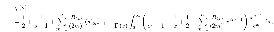
25.5.7
, .
…
►
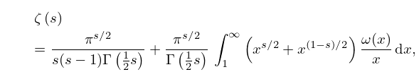
25.5.13
,
…
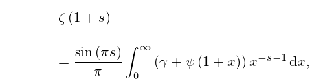
►In (25.5.15)–(25.5.19), , is the digamma function, and is Euler’s constant (§5.2).
…
►
25.5.17
…
►
25.5.19
.
…
18: Bibliography D
…
►
Recherches analytiques sur la théorie des nombres premiers. Deuxième partie. Les fonctions de Dirichlet et les nombres premiers de la forme linéaire
.
Ann. Soc. Sci. Bruxelles 20, pp. 281–397 (French).
…
►
Sums of products of Bernoulli numbers.
J. Number Theory 60 (1), pp. 23–41.
…
►
A simple sum formula for Clebsch-Gordan coefficients.
Lett. Math. Phys. 5 (3), pp. 207–211.
…
►
Complex zeros of cylinder functions.
Math. Comp. 20 (94), pp. 215–222.
…
►
Uniform asymptotic expansions for Whittaker’s confluent hypergeometric functions.
SIAM J. Math. Anal. 20 (3), pp. 744–760.
…
19: 18.39 Applications in the Physical Sciences
…
►As in classical dynamics this sum is the total energy of the one particle system.
…
►The spectrum is mixed as in §1.18(viii), with the discrete eigenvalues given by (18.39.18) and the continuous eigenvalues by () with corresponding eigenfunctions expressed in terms of Whittaker functions (13.14.3).
…
►The fact that both the eigenvalues of (18.39.31) and the scaling of the co-ordinate in the eigenfunctions, (18.39.30), depend on the sum
leads to the substitution
…
►Derivations of (18.39.42) appear in Bethe and Salpeter (1957, pp. 12–20), and Pauling and Wilson (1985, Chapter V and Appendix VII), where the derivations are based on (18.39.36), and is also the notation of Piela (2014, §4.7), typifying the common use of the associated Coulomb–Laguerre polynomials in theoretical quantum chemistry.
…
►The fact that non- continuum scattering eigenstates may be expressed in terms or (infinite) sums of functions allows a reformulation of scattering theory in atomic physics wherein no non- functions need appear.
…
