§1.18 Linear Second Order Differential Operators and Eigenfunction Expansions
Contents
- §1.18(i) Hilbert spaces
- §1.18(ii) spaces on intervals in
- §1.18(iii) Linear Operators on a Hilbert Space
- §1.18(iv) Formally Self-adjoint Linear Second Order Differential Operators
- §1.18(v) Point Spectra and Eigenfunction Expansions
- §1.18(vi) Continuous Spectra and Eigenfunction Expansions: Simple Cases
- §1.18(vii) Continuous Spectra: More General Cases
- §1.18(viii) Mixed Spectra and Eigenfunction Expansions
- §1.18(ix) Mathematical Background
- §1.18(x) Literature
A survey is given of the formal spectral theory of second order differential operators, typical results being presented in §1.18(i) through §1.18(viii). The various types of spectra and the corresponding eigenfunction expansions are illustrated by examples. These are based on the Liouville normal form of (1.13.29). A more precise mathematical discussion then follows in §1.18(ix).
§1.18(i) Hilbert spaces
A complex linear vector space is called an inner product space if an inner product is defined for all with the properties: (i) is complex linear in ; (ii) ; (iii) ; (iv) if then . With norm defined by
| 1.18.1 | |||
becomes a normed linear vector space. If then is normalized. Two elements and in are orthogonal if . A (finite or countably infinite, generalizing the definition of (1.2.40)) set is an orthonormal set if the are normalized and pairwise orthogonal.
An inner product space is called a Hilbert space if every Cauchy sequence in (i.e., ) converges in norm to some , i.e., . For an orthonormal set in a Hilbert space Bessel’s inequality holds:
| 1.18.2 | |||
where and
| 1.18.3 | |||
A Hilbert space is separable if there is an (at most countably infinite) orthonormal set in such that for every
| 1.18.4 | |||
where is given by (1.18.3). Such orthonormal sets are called complete. By (1.18.4)
| 1.18.5 | |||
Conversely, if complex numbers satisfy (1.18.5) then there is a unique such that (1.18.3) holds and can be given by
| 1.18.6 | |||
where the infinite sum means convergence in norm,
| 1.18.7 | |||
The standard example of an (infinite dimensional) separable Hilbert space is the space with elements such that
| 1.18.8 | |||
The inner product of and is
| 1.18.9 | |||
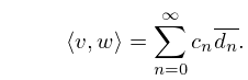
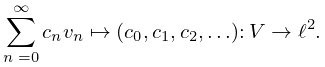
Every infinite dimensional separable Hilbert space can be made isomorphic to by choosing a complete orthonormal set in . Then an isomorphism is given by
| 1.18.10 | |||
General references for this subsection include Friedman (1990, pp. 4–6), Shilov (2013, pp. 249–256), Riesz and Sz.-Nagy (1990, Ch. 5, §82).
§1.18(ii) spaces on intervals in
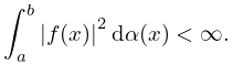
Let or or or be a (possibly infinite, or semi-infinite) interval in . For a Lebesgue–Stieltjes measure on let be the space of all Lebesgue–Stieltjes measurable complex-valued functions on which are square integrable with respect to ,
| 1.18.11 | |||
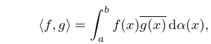
Functions for which are identified with each other. The space becomes a separable Hilbert space with inner product
| 1.18.12 | |||
thus generalizing the inner product of (1.18.9). When is absolutely continuous, i.e. , see §1.4(v), where the nonnegative weight function is Lebesgue measurable on . In this section we will only consider the special case , so ; in which case .
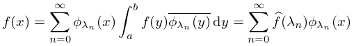
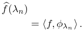
Assume that is an orthonormal basis of . The formulas in §1.18(i) are then:
| 1.18.13 | |||
| , | |||
| 1.18.14 | |||
| , | |||
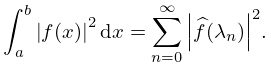
| 1.18.15 | |||
where the limit has to be understood in the sense of convergence in the mean:
| 1.18.16 | |||
Often circumstances allow rather stronger statements, such as uniform convergence, or pointwise convergence at points where is continuous, with convergence to if is an isolated point of discontinuity.
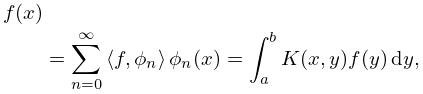
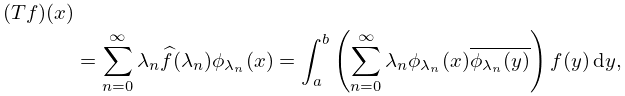
We can rewrite (1.18.15), together with (1.18.13), formally as
| 1.18.17 | |||
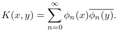
where the integral kernel is given by
| 1.18.18 | |||
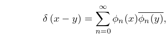
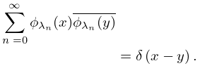
Thus, in the notation of §1.17, we have an expansion
| 1.18.19 | |||
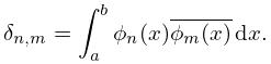
of the Dirac delta distribution. Equation (1.18.19) is often called the completeness relation. The analogous orthonormality is
| 1.18.20 | |||
§1.18(iii) Linear Operators on a Hilbert Space
Bounded and Unbounded Linear Operators
A linear operator on a (complex) linear vector space is a map such that
| 1.18.21 | |||
| , . | |||
In the following let be a Hilbert space. A linear operator on is bounded with norm if
| 1.18.22 | |||
More generally, a linear operator on needs not be defined on all of , but only on a linear subspace of which is called the domain of . Then is a linear map. Assume that is dense in , i.e., for each there is a sequence in such that as . If is finite then is bounded, and extends uniquely to a bounded linear operator on . If the supremum is , then is an unbounded linear operator on .
Self-Adjoint and Symmetric Operators
If is a bounded linear operator on then its adjoint is the bounded linear operator such that, for ,
| 1.18.23 | |||
The operator is called self-adjoint if , and referred to as symmetric if (1.18.23) holds for in the dense domain of . There is also a notion of self-adjointness for unbounded operators, see §1.18(ix). One then needs a self-adjoint extension of a symmetric operator to carry out its spectral theory in a mathematically rigorous manner.
An essential feature of such symmetric operators is that their eigenvalues are real, and eigenfunctions
| 1.18.24 | |||
, corresponding to distinct eigenvalues, are orthogonal: i.e., , for . If an eigenvalue has multiplicity , the eigenfunctions may always be orthogonalized in this degenerate sub-space.
Formally Self-Adjoint and Self-Adjoint Differential Operators: Self-Adjoint Extensions
Focus is now placed on second order differential operators as these are the subject of the remainder of §1.18.
Consider the second order differential operator acting on real functions of in the finite interval
| 1.18.25 | |||
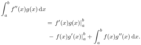
and functions , assumed real for the moment. The adjoint of does satisfy where . We integrate by parts twice giving:
| 1.18.26 | |||
Ignoring the boundary value terms it follows that
| 1.18.27 | |||
and thus is said to be formally self adjoint.
For to be actually self adjoint it is necessary to also show that , as it is often the case that and have different domains, see Friedman (1990, p 148) for a simple example of such differences involving the differential operator .
This question may be rephrased by asking: do and satisfy the same boundary conditions which are needed to fully specify the solutions of a second order linear differential equation? A simple example is the choice , and , this being only one of many. This insures the vanishing of the boundary terms in (1.18.26), and also is a choice which indicates that , as and satisfy the same boundary conditions and thus define the same domains. Thus is indeed self adjoint.
Other choices of boundary conditions, identical for and , and which also lead to the vanishing of the boundary terms in (1.18.26), each lead to a distinct self adjoint extension of . The nature of these extensions for unbounded intervals such as , and unbounded operators on them, are the subject of §1.18(ix).
§1.18(iv) Formally Self-adjoint Linear Second Order Differential Operators
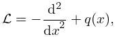
Let be a finite or infinite open interval in . Consider on the linear formally self-adjoint second order differential operator
| 1.18.28 | |||
with real and continuous, unless otherwise noted.
Eigenvalues and eigenfunctions of , self-adjoint extensions of with well defined boundary conditions, and utilization of such eigenfunctions for expansion of wide classes of functions, will be the focus of the remainder of this section.
The special form of (1.18.28) is especially useful for applications in physics, as the connection to non-relativistic quantum mechanics is immediate: being proportional to the kinetic energy operator for a single particle in one dimension, being proportional to the potential energy, often written as , of that same particle, and which is simply a multiplicative operator. The sum of the kinetic and potential energies give the quantum Hamiltonian, or energy operator; often also referred to as a Schrödinger operator. Other applications follow from the fact that is suitable for describing vibrations, especially standing waves, which arise in many parts of engineering and the physical sciences, see Birkhoff and Rota (1989, §§10.3 and 10.16). See §18.39(i).
In what follows will be taken to be a self adjoint extension of following the discussion ending the prior sub-section. For we can take , with appropriate boundary conditions, and with compact support if is bounded, which space is dense in , and for unbounded require that possible non- eigenfunctions of (1.18.28), with real eigenvalues, are non-zero but bounded on open intervals, including .
Stated informally, the spectrum of is the set of it’s eigenvalues, these being real as is self-adjoint. These sets may be discrete, continuous, or a combination of both, as discussed in the following three subsections. Should an eigenvalue correspond to more than a single linearly independent eigenfunction, namely a multiplicity greater than one, all such eigenfunctions will always be implied as being part of any sums or integrals over the spectrum.
§1.18(v) Point Spectra and Eigenfunction Expansions
General Results
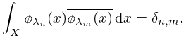
Let be a self-adjoint extension of differential operator of the form (1.18.28) and assume has a complete set of eigenfunctions, , this latter being an appropriate sub-set of , or, in some cases itself, with real eigenvalues . These eigenvalues will be assumed distinct, i.e., of unit multiplicity, unless otherwise stated. The point, or discrete spectrum of is then given by . The eigenfunctions form a complete orthogonal basis in , and we can take the basis as orthonormal:
| 1.18.29 | |||
and completeness implies
| 1.18.30 | |||
Now formulas (1.18.13)–(1.18.20) apply. For , has the eigenfunction expansion, following directly from (1.18.17)–(1.18.19),
| 1.18.31 | |||
where
| 1.18.32 | |||
Further
| 1.18.33 | |||
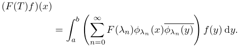
Spectral expansions of , and of functions of , these being expansions of and in terms of the eigenvalues and eigenfunctions summed over the spectrum, then follow:
| 1.18.34 | |||
| 1.18.35 | |||
Example 1: Three Simple Cases where ,
Possible eigenfunctions of being , , , consider three cases, which illustrate the importance of boundary conditions.
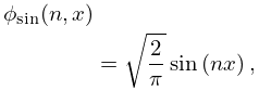
Case 1: . The normalized eigenfunctions on are
| 1.18.36 | |||
with , .
Case 2: . The normalized eigenfunctions on are
| 1.18.37 | |||
| , | |||
with , .
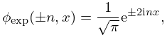
Case 3: Periodic Boundary Conditions: and . The normalized eigenfunctions on are
| 1.18.38 | |||
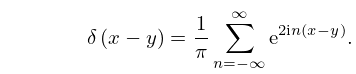
with , , with all eigenvalues, for , having multiplicity two, as changing the sign of changes the eigenfunction but not the eigenvalue, and multiplicity one for . Letting run from to this multiplicity change is automatically included:
| 1.18.39 | |||
This may be compared to (1.17.21), the resulting Fourier, or eigenfunction, expansion
| 1.18.40 | |||
where = , being that of (1.8.3) and (1.8.4). The eigenfunction expansions of (1.8.1) and (1.8.2) follow from Cases 1, 2, above.
Hermite’s Differential Equation,
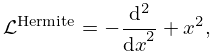
The space is now the full real line, . Writing Hermite’s differential equation (see Tables 18.3.1 and 18.8.1) in the form above, the eigenfunctions are ( a Hermite polynomial, ), with eigenvalues , for the differential operator
| 1.18.41 | |||
| . | |||
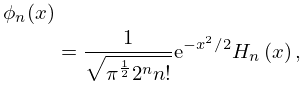
Applying equations (1.18.29) and (1.18.30), the complete set of normalized eigenfunctions being
| 1.18.42 | |||
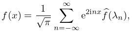
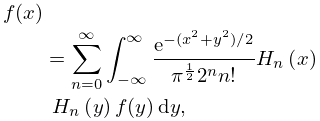
(1.18.31) becomes
| 1.18.43 | |||
for and piece-wise continuous, with convergence as discussed in §1.18(ii).
§1.18(vi) Continuous Spectra and Eigenfunction Expansions: Simple Cases
General Results
Eigenfunctions corresponding to the continuous spectrum are non- functions. Let be the self adjoint extension of a formally self-adjoint differential operator of the form (1.18.28) on an unbounded interval , which we will take as , and assume that monotonically as , and that the eigenfunctions are non-vanishing but bounded in this same limit. Assume has no point spectrum, i.e., has no eigenfunctions in , then the spectrum of consists only of a continuous spectrum, referred to as . In this subsection it is assumed that . This will be generalized, along with the choice of , in §1.18(vii).
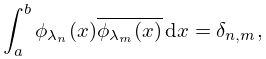
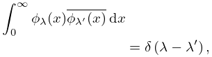
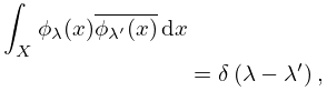
Orthogonality and normalization may then be chosen such that analogous to (1.18.19) and (1.18.20), we have
| 1.18.44 | |||
| , | |||
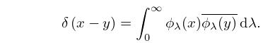
and completeness relation
| 1.18.45 | |||
See Friedman (1990, pp. 233–252) for elementary discussions of both equations and the normalization process; and also the references in §1.18(ix).
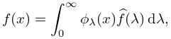
Now formulas (1.18.13)–(1.18.20) apply. For , has the eigenfunction expansion, analogous to that of (1.18.33),
| 1.18.46 | |||
where
| 1.18.47 | |||
Further,
| 1.18.48 | |||
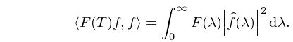
The analog of (1.18.34) is
| 1.18.49 | |||
and that of (1.18.35) is
| 1.18.50 | |||
This implies
| 1.18.51 | |||
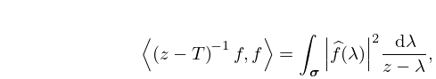
In particular, this holds for ,
| 1.18.52 | |||
| , , | |||
this being a matrix element of the resolvent , this being a key quantity in many parts of physics and applied math, quantum scattering theory being a simple example, see Newton (2002, Ch. 7). Then
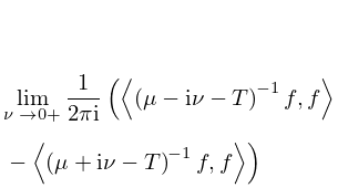
| 1.18.53 | |||
gives for , and otherwise. This is the discontinuity across the branch cut in (1.18.52) , from below to above the cut, divided by . See Newton (2002, §§7.1 and 7.3).
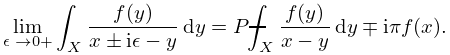
More generally, for , , see (1.4.24),
| 1.18.54 | |||
Example 1: Bessel–Hankel Transform,
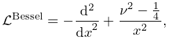
By Bessel’s differential equation in the form (10.13.1) we have the functions (, for see §10.2(ii)) as eigenfunctions with eigenvalue of the self-adjoint extension of the differential operator
| 1.18.55 | |||
| . | |||
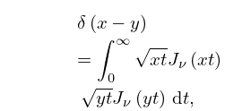
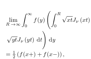
Applying the representation (1.17.13), now symmetrized as in (1.17.14), as ,
| 1.18.56 | |||
| , . | |||
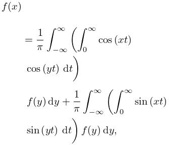
Example 2: Sine and Cosine Transforms,
§1.18(vii) Continuous Spectra: More General Cases
More generally, continuous spectra may occur in sets of disjoint finite intervals , often called bands, when is periodic, see Ashcroft and Mermin (1976, Ch 8) and Kittel (1996, Ch 7). Should be bounded but random, leading to Anderson localization, the spectrum could range from being a dense point spectrum to being singular continuous, see Simon (1995), Avron and Simon (1982); a good general reference being Cycon et al. (2008, Ch. 9 and 10). For example, replacing of (28.2.1) by , gives an almost Mathieu equation which for appropriate has such properties.
§1.18(viii) Mixed Spectra and Eigenfunction Expansions
In general, operators being formally self-adjoint second order differential operators of the form (1.18.28), with unbounded, will have both a continuous and a point spectrum, and thus, correspondingly, eigenfunctions as in §1.18(vi) and eigenfunctions as in §1.18(v). We assume a continuous spectrum , and a finite or countably infinite point spectrum with elements . In what follows, integrals over the continuous parts of the spectrum will be denoted by , and sums over the discrete spectrum by , with denoting the full spectrum. It is to be noted that if any of the have degenerate sub-spaces, that is subspaces of orthogonal eigenfunctions with identical eigenvalues, that in the expansions below all such distinct eigenfunctions are to be included. Then orthogonality and normalization relations are
| 1.18.60 | |||
| , | |||
| 1.18.61 | |||
| , | |||
| 1.18.62 | |||
| , , | |||
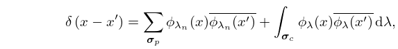
compare (1.18.29) and (1.18.44). The formal completeness relation is now
| 1.18.63 | |||
| , | |||
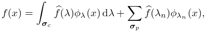
compare (1.18.30) and (1.18.45), and the eigenfunction expansions are of the form
| 1.18.64 | |||
| . | |||
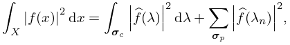
Note that the notations of (1.18.32) and (1.18.47) are used to distinguish the contributions from the discrete and continuous parts of the spectrum. Then
| 1.18.65 | |||
| . | |||
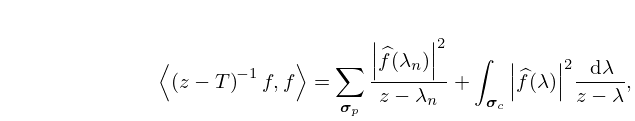
The analogs of (1.18.49)–(1.18.52) may be written in a similar fashion each now including contributions from both the discrete and continuous parts of the spectrum, as in (1.18.65). Showing one, representative, example: the analog of (1.18.52) is now
| 1.18.66 | |||
| , . | |||
This representation has poles with residues at the discrete eigenvalues and a branch cut along with discontinuity, from below to above the cut, , as in (1.18.53), see Newton (2002, §7.1.1).
Note that the integral in (1.18.66) is not singular if approached separately from above, or below, the real axis: in fact analytic continuation from the upper half of the complex plane, across the cut, and onto higher Riemann Sheets can access complex poles with singularities at discrete energies corresponding to quantum resonances, or decaying quantum states with lifetimes proportional to . For this latter see Simon (1973), and Reinhardt (1982); wherein advantage is taken of the fact that although branch points are actual singularities of an analytic function, the location of the branch cuts are often at our disposal, as they are not singularities of the function, but simply arbitrary lines to keep a function single valued, and thus only singularities of a specific representation of that analytic function. This is accomplished by the variable change , in , which rotates the continuous spectrum and the branch cut of (1.18.66) into the lower half complex plain by the angle , with respect to the unmoved branch point at ; thus, providing access to resonances on the higher Riemann sheet should be large enough to expose them. This dilatation transformation, which does require analyticity of in (1.18.28), or an analytic approximation thereto, leaves the poles, corresponding to the discrete spectrum, invariant, as they are, as is the branch point, actual singularities of .
Example 1: In one and two dimensions any with a ‘Dip, or Well’ has a partly discrete spectrum
Suppose that is the whole real line in one dimension, and that , in (1.18.28) has (non-oscillatory) limits of at both , and thus a continuous spectrum on . What then is the condition on to insure the existence of at least a single eigenvalue in the point spectrum? The discussions of §1.18(vi) imply that if then there is only a continuous spectrum. Surprisingly, if on any interval on the real line, even if positive elsewhere, as long as , see Simon (1976, Theorem 2.5), then there will be at least one eigenfunction with a negative eigenvalue, with corresponding eigenfunction. Thus, and this is a case where is not continuous, if , , there will be an eigenfunction localized in the vicinity of , with a negative eigenvalue, thus disjoint from the continuous spectrum on . Similar results hold for two, but not higher, dimensional quantum systems. See Brownstein (2000) and Yang and de Llano (1989) for numerical examples, based on variational calculations, and Simon (1976) and Chadan et al. (2003) for rigorous mathematical discussion.
Example 2: Radial 3D Schrödinger operators, including the Coulomb potential
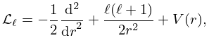
Consider formally self-adjoint operators of the form
| 1.18.67 | |||
| , as , | |||
which appear in the quantum theory of binding or scattering of a particle in a spherically symmetric potential in three dimensions, and where . The bound states are in the negative energy discrete spectrum, and the scattering states are in the positive energy continuous spectrum, , or, said more simply, in the continuum. See §18.39 for discussion of Schrödinger equations and operators. For fixed angular momentum the appropriate self-adjoint extension of the above operator may have both a discrete spectrum of negative eigenvalues , with corresponding eigenfunctions , and also a continuous spectrum , with Dirac-delta normalized eigenfunctions , also with measure . Unlike in the example in the paragraph above, in 3-dimensions a “dip below zero, or a potential well” in does not always correspond to the existence of a discrete part of the spectrum. The well must be deep and broad enough to allow existence of such discrete states. The number, , of discrete states depends on the nature of , as well as , and, again, must vanish as , corresponding to the traditionally assumed start of the energy continuum at . In unusual cases , even for all , such as in the case of the Schrödinger–Coulomb problem () discussed in §18.39 and §33.14, where the point spectrum actually accumulates at the onset of the continuum at , implying an essential singularity, as well as a branch point, in matrix elements of the resolvent, (1.18.66). See Bethe and Salpeter (1977, Ch. 1, (4.12)–(4.13)) for the resulting transform pair in this case.
§1.18(ix) Mathematical Background
Self-Adjoint Operators
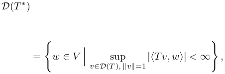
If is an unbounded linear operator on a Hilbert space with dense domain then the adjoint of is the linear operator with domain
| 1.18.68 | |||
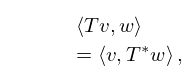
such that
| 1.18.69 | |||
| , . | |||
A linear operator with dense domain is called symmetric if
| 1.18.70 | |||
| . | |||
If is symmetric then , i.e., and for . Then also , where . If then is essentially self-adjoint and if then is self-adjoint.
Spectrum of an Operator
Let be a linear operator on with dense domain and with range . Such an operator is called injective if, for any in its domain, implies that . The resolvent set consists of all such that (i) is injective, (ii) is dense in , (iii) the resolvent is bounded. The spectrum is the complement in of . The spectrum is the disjoint union of three sets:
-
1.
The point spectrum . It consists of all for which is not injective, or equivalently, for which is an eigenvalue of , i.e., for some .
-
2.
The continuous spectrum . It consists of all for which is injective and has dense range, but is not bounded.
-
3.
The residual spectrum. It consists of all for which is injective, but does not have dense range.
If is a bounded operator then its spectrum is a closed bounded subset of . If is self-adjoint (bounded or unbounded) then is a closed subset of and the residual spectrum is empty. Note that eigenfunctions for distinct (necessarily real) eigenvalues of a self-adjoint operator are mutually orthogonal. If an eigenvalue is of multiplicity greater than then an orthonormal basis of eigenfunctions can be given for the eigenspace.
Self-adjoint extensions of a symmetric Operator
Let be a symmetric operator on a Hilbert space , so is dense in and . For let be the -eigenspace of , i.e., is the linear subspace of consisting of all for which . Then is constant for and also constant for . Put () and (), the deficiency indices for . Then has self-adjoint extensions iff . We have a direct sum of linear spaces: . Assume . Then any self-adjoint extension of is determined by a linear isometry and it is the restriction of to .
Self-adjoint extensions of (1.18.28) and the Weyl alternative
For a formally self-adjoint second order differential operator , such as that of (1.18.28), the space can be seen to consist of all such that the distribution can be identified with a function in , which is the function . Then, for , iff is an ordinary solution (i.e., ) of which is moreover in . Thus has dimension 0, 1 or 2. Also, because is real-valued, iff . So has self-adjoint extensions with deficiency indices , or or . Pick . Let be the deficiency indices for restricted to , and the ones for restricted to . Then and are independent of . By Weyl’s alternative equals either 1 (the limit point case) or 2 (the limit circle case), and similarly for . The two (equal) deficiency indices of are then equal to . A boundary value for the end point is a linear form on of the form
| 1.18.71 | |||
| , | |||
where and are given functions on , and where the limit has to exist for all . Then, if the linear form is nonzero, the condition is called a boundary condition at . Boundary values and boundary conditions for the end point are defined in a similar way. If then there are no nonzero boundary values at ; if then the above boundary values at form a two-dimensional class. Similarly at . Any self-adjoint extension of can be obtained by restricting to those for which, if , for a chosen at and, if , for a chosen at .
Spectral expansions and self-adjoint extensions
The above results, especially the discussions of deficiency indices and limit point and limit circle boundary conditions, lay the basis for further applications. The reader is referred to Coddington and Levinson (1955), Friedman (1990, Ch. 3), Titchmarsh (1962a), and Everitt (2005b, pp. 45–74) and Everitt (2005a, pp. 272–331), for detailed methods and results.
§1.18(x) Literature
The materials developed here follow from the extensions of the Sturm–Liouville theory of second order ODEs as developed by Weyl, to include the limit point and limit circle singular cases. This work is well overviewed by Coddington and Levinson (1955, Ch. 9), and then applied in detail by Titchmarsh (1946), Titchmarsh (1962a), Titchmarsh (1958), and Levitan and Sargsjan (1975) which also connects the Weyl theory to the relevant functional analysis. In parallel, similar, and more general formulations have grown out of functional analysis itself, as in the work of Stone (1990), Rudin (1973), Reed and Simon (1980), Reed and Simon (1975), Reed and Simon (1978), Reed and Simon (1979), Cycon et al. (2008), Dunford and Schwartz (1988, Ch. XIII), Hall (2013, pp. 127-223). Friedman (1990) provides a useful introduction to both approaches; as does the conference proceeding Amrein et al. (2005), overviewing the combination of Sturm–Liouville theory and Hilbert space theory. See, in particular, the overview Everitt (2005b, pp. 45–74), and the uniformly annotated listing of solved Sturm–Liouville problems in Everitt (2005a, pp. 272–331), each with their limit point, or circle, boundary behaviors categorized.
