.%E4%B8%96%E7%95%8C%E6%9D%AF%E4%BD%93%E5%BD%A9%E4%B8%B2%E4%B9%B0%E3%80%8E%E7%BD%91%E5%9D%80%3Amxsty.cc%E3%80%8F.%E9%99%AA%E7%9C%8B%E4%B8%96%E7%95%8C%E6%9D%AF%E5%A5%B3%E5%AD%A9.m6q3s2-2022%E5%B9%B411%E6%9C%8829%E6%97%A57%E6%97%B60%E5%88%869%E7%A7%92.%E5%AD%97%E7%AC%A6%3Ewcamcs

SearchAdvancedHelp

(0.058 seconds)

11—20 of 768 matching pages

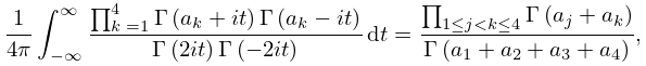
11: 5.13 Integrals

… ►

5.13.4 $${\int }_{-\mathrm{\infty }}^{\mathrm{\infty }}\frac{dt}{\mathrm{\Gamma }\left(a+t\right)\mathrm{\Gamma }\left(b+t\right)\mathrm{\Gamma }\left(c-t\right)\mathrm{\Gamma }\left(d-t\right)}=\frac{\mathrm{\Gamma }\left(a+b+c+d-3\right)}{\mathrm{\Gamma }\left(a+c-1\right)\mathrm{\Gamma }\left(a+d-1\right)\mathrm{\Gamma }\left(b+c-1\right)\mathrm{\Gamma }\left(b+d-1\right)},$$ $\mathrm{\Re }\left(a+b+c+d\right)>3$.

ⓘ

Symbols:

$\mathrm{\Gamma }\left(z\right)$: gamma function, $dx$: differential of $x$ , $\int$: integral, $\mathrm{\Re }$: real part, $a$: real or complex variable and $b$: real or complex variable

Referenced by:

§5.13

Permalink:

http://dlmf.nist.gov/5.13.E4

Encodings:

pMML, png, TeX

See also:

Annotations for §5.13, §5.13 and Ch.5

… ►

5.13.5 $\mathrm{\Re }\left(a_k\right)>0$, $k=1,2,3,4$.

ⓘ

Symbols:

$\mathrm{\Gamma }\left(z\right)$: gamma function, $\pi$: the ratio of the circumference of a circle to its diameter, $dx$: differential of $x$ , $\mathrm{i}$: imaginary unit, $\int$: integral, $\mathrm{\Re }$: real part, $j$: nonnegative integer, $k$: nonnegative integer and $a$: real or complex variable

Referenced by:

§5.13

Permalink:

http://dlmf.nist.gov/5.13.E5

Encodings:

pMML, png, TeX

See also:

Annotations for §5.13, §5.13 and Ch.5

…

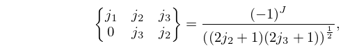
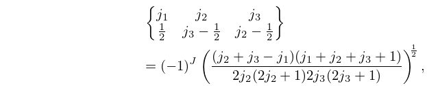
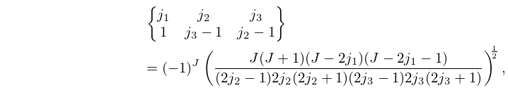
12: 34.5 Basic Properties: $\mathit{6}j$ Symbol

… ►

34.5.1

ⓘ

Symbols:

: $\mathit{6}j$ symbol, $j,j_r$: non-negative integers or non-negative integers plus one half. and $J$: sum

Permalink:

http://dlmf.nist.gov/34.5.E1

Encodings:

pMML, png, TeX

See also:

Annotations for §34.5(i), §34.5 and Ch.34

►

34.5.2

ⓘ

Symbols:

: $\mathit{6}j$ symbol, $j,j_r$: non-negative integers or non-negative integers plus one half. and $J$: sum

Permalink:

http://dlmf.nist.gov/34.5.E2

Encodings:

pMML, png, TeX

See also:

Annotations for §34.5(i), §34.5 and Ch.34

►

34.5.3

ⓘ

Symbols:

: $\mathit{6}j$ symbol, $j,j_r$: non-negative integers or non-negative integers plus one half. and $J$: sum

Permalink:

http://dlmf.nist.gov/34.5.E3

Encodings:

pMML, png, TeX

See also:

Annotations for §34.5(i), §34.5 and Ch.34

►

34.5.4

ⓘ

Symbols:

: $\mathit{6}j$ symbol, $j,j_r$: non-negative integers or non-negative integers plus one half. and $J$: sum

Permalink:

http://dlmf.nist.gov/34.5.E4

Encodings:

pMML, png, TeX

See also:

Annotations for §34.5(i), §34.5 and Ch.34

… ►For further recursion relations see Varshalovich et al. (1988, §9.6) and Edmonds (1974, pp. 98–99). …

13: 27.2 Functions

… ►

27.2.9 $$d\left(n\right)=\sum _{d|n}1$$

ⓘ

Symbols:

$d_k\left(n\right)$: divisor function, $d$: positive integer and $n$: positive integer

A&S Ref:

24.3.3 I.A

Permalink:

http://dlmf.nist.gov/27.2.E9

Encodings:

pMML, png, TeX

See also:

Annotations for §27.2(i), §27.2 and Ch.27

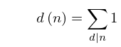
… ►It is the special case $k=2$ of the function $d_k\left(n\right)$ that counts the number of ways of expressing $n$ as the product of $k$ factors, with the order of factors taken into account. …Note that ${\sigma }_0\left(n\right)=d\left(n\right)$. … ►Table 27.2.2 tabulates the Euler totient function $\varphi \left(n\right)$, the divisor function $d\left(n\right)$ ($={\sigma }_0(n)$), and the sum of the divisors $\sigma (n)$ ($={\sigma }_1(n)$), for $n=1(1)52$. … ►

Table 27.2.2: Functions related to division.

► ►►►

$n$	$\varphi \left(n\right)$	$d\left(n\right)$	$\sigma \left(n\right)$	$n$	$\varphi \left(n\right)$	$d\left(n\right)$	$\sigma \left(n\right)$	$n$	$\varphi \left(n\right)$	$d\left(n\right)$	$\sigma \left(n\right)$	$n$	$\varphi \left(n\right)$	$d\left(n\right)$	$\sigma \left(n\right)$
…
3	2	2	4	16	8	5	31	29	28	2	30	42	12	8	96
…

►

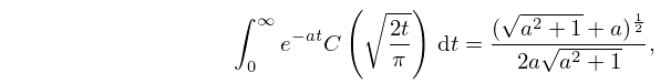
14: 7.14 Integrals

… ►

7.14.1 $${\int }_0^{\mathrm{\infty }}{\mathrm{e}}^{2\mathrm{i}at}\mathrm{erfc}\left(bt\right)dt=\frac{1}{a\sqrt{\pi }}F\left(\frac{a}{b}\right)+\frac{\mathrm{i}}{2a}\left(1-{\mathrm{e}}^{-{(a/b)}^2}\right),$$ $a\in ℂ$, .

ⓘ

Symbols:

$F\left(z\right)$: Dawson’s integral, $\pi$: the ratio of the circumference of a circle to its diameter, $\mathrm{erfc}z$: complementary error function, $ℂ$: complex plane, $dx$: differential of $x$ , $\in$: element of, $\mathrm{e}$: base of natural logarithm, $\mathrm{i}$: imaginary unit, $\int$: integral and $\mathrm{ph}$: phase

A&S Ref:

7.4.18 (in different form)

Referenced by:

§7.14(i)

Permalink:

http://dlmf.nist.gov/7.14.E1

Encodings:

pMML, png, TeX

See also:

Annotations for §7.14(i), §7.14(i), §7.14 and Ch.7

… ►

7.14.5 $${\int }_0^{\mathrm{\infty }}{\mathrm{e}}^{-at}C\left(t\right)dt=\frac{1}{a}\mathrm{f}\left(\frac{a}{\pi }\right),$$ $\mathrm{\Re }a>0$,

ⓘ

Symbols:

$\mathrm{f}\left(z\right)$: auxiliary function for Fresnel integrals, $C\left(z\right)$: Fresnel integral, $\pi$: the ratio of the circumference of a circle to its diameter, $dx$: differential of $x$ , $\mathrm{e}$: base of natural logarithm, $\int$: integral and $\mathrm{\Re }$: real part

Keywords:

Laplace transform

A&S Ref:

7.4.27 (in different notation)

Referenced by:

§7.14(ii)

Permalink:

http://dlmf.nist.gov/7.14.E5

Encodings:

pMML, png, TeX

See also:

Annotations for §7.14(ii), §7.14(ii), §7.14 and Ch.7

… ►

7.14.7 $${\int }_0^{\mathrm{\infty }}{\mathrm{e}}^{-at}C\left(\sqrt{\frac{2t}{\pi }}\right)dt=\frac{{(\sqrt{a^2+1}+a)}^{\frac{1}{2}}}{2a\sqrt{a^2+1}},$$ $\mathrm{\Re }a>0$,

ⓘ

Symbols:

$C\left(z\right)$: Fresnel integral, $\pi$: the ratio of the circumference of a circle to its diameter, $dx$: differential of $x$ , $\mathrm{e}$: base of natural logarithm, $\int$: integral and $\mathrm{\Re }$: real part

Keywords:

Laplace transform

A&S Ref:

7.4.29 in modified form

Referenced by:

§7.14(ii)

Permalink:

http://dlmf.nist.gov/7.14.E7

Encodings:

pMML, png, TeX

See also:

Annotations for §7.14(ii), §7.14(ii), §7.14 and Ch.7

… ►For collections of integrals see Apelblat (1983, pp. 131–146), Erdélyi et al. (1954a, vol. 1, pp. 40, 96, 176–177), Geller and Ng (1971), Gradshteyn and Ryzhik (2000, §§5.4 and 6.28–6.32), Marichev (1983, pp. 184–189), Ng and Geller (1969), Oberhettinger (1974, pp. 138–139, 142–143), Oberhettinger (1990, pp. 48–52, 155–158), Oberhettinger and Badii (1973, pp. 171–172, 179–181), Prudnikov et al. (1986b, vol. 2, pp. 30–36, 93–143), Prudnikov et al. (1992a, §§3.7–3.8), and Prudnikov et al. (1992b, §§3.7–3.8). …

15: Bibliography F

… ►

Tables of Elliptic Integrals of the First, Second, and Third Kind. Technical report Technical Report ARL 64-232, Aerospace Research Laboratories, Wright-Patterson Air Force Base, Ohio.

ⓘ

Notes:

Reviewed in Math. Comp. v. 1919(1965)509. Table erratum: Math. Comp. v. 20 (1966), no. 96, pp. 639-640.

Referenced by:

§19.37(ii), §19.37(ii), §19.37(iii), §19.37(iii), §19.37(iii).

Encodings:

BibTeX

… ►

Algorithm 309. Gamma function with arbitrary precision. Comm. ACM 10 (8), pp. 511–512.

ⓘ

External Links:

ISSN 0001-0782, Document

Referenced by:

§5.24(ii).

Encodings:

BibTeX

… ►

Diffraction of radio waves around the earth’s surface. Acad. Sci. USSR. J. Phys. 9, pp. 255–266.

ⓘ

External Links:

MathReview, ZentralBlatt

Referenced by:

§9.1, Notations U, Notations V.

Encodings:

BibTeX

… ►

Travel time surface of a transverse cusp caustic produced by reflection of acoustical transients from a curved metal surface. J. Acoust. Soc. Amer. 95 (2), pp. 650–660.

ⓘ

External Links:

Document

Referenced by:

§36.14(iv).

Encodings:

BibTeX

… ►

Evaluation, design and extrapolation methods for optical signals, based on use of the prolate functions. In Progress in Optics, E. Wolf (Ed.), Vol. 9, pp. 311–407.

ⓘ

Referenced by:

§30.15(i), §30.15(ii), §30.15(iii), §30.15(iv), §30.15(v), §30.15(v).

Encodings:

BibTeX

…

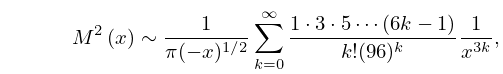
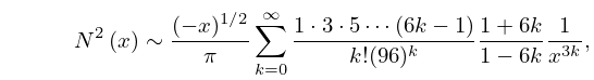
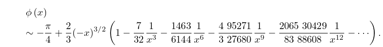
16: 9.8 Modulus and Phase

… ►In terms of Bessel functions, and with $\xi =\frac{2}{3}{|x|}^{3/2}$, … ►

9.8.20 $$M^2\left(x\right)\sim \frac{1}{\pi {(-x)}^{1/2}}\sum _{k=0}^{\mathrm{\infty }}\frac{1\cdot 3\cdot 5\mathrm{\cdots }(6k-1)}{k!{(96)}^k}\frac{1}{x^{3k}},$$

ⓘ

Symbols:

$\sim$: Poincaré asymptotic expansion, $\pi$: the ratio of the circumference of a circle to its diameter, $!$: factorial (as in $n!$), $M\left(z\right)$: Airy modulus function and $x$: real variable

Proof sketch:

Combine (9.8.9)–(9.8.12) with §10.18(iii)

Referenced by:

§9.8(iv)

Permalink:

http://dlmf.nist.gov/9.8.E20

Encodings:

pMML, png, TeX

See also:

Annotations for §9.8(iv), §9.8 and Ch.9

►

9.8.21 $$N^2\left(x\right)\sim \frac{{(-x)}^{1/2}}{\pi }\sum _{k=0}^{\mathrm{\infty }}\frac{1\cdot 3\cdot 5\mathrm{\cdots }(6k-1)}{k!{(96)}^k}\frac{1+6k}{1-6k}\frac{1}{x^{3k}},$$

ⓘ

Symbols:

$\sim$: Poincaré asymptotic expansion, $\pi$: the ratio of the circumference of a circle to its diameter, $!$: factorial (as in $n!$), $N\left(z\right)$: Airy modulus function and $x$: real variable

Proof sketch:

Combine (9.8.9)–(9.8.12) with §10.18(iii)

Referenced by:

§9.8(iv)

Permalink:

http://dlmf.nist.gov/9.8.E21

Encodings:

pMML, png, TeX

See also:

Annotations for §9.8(iv), §9.8 and Ch.9

►

9.8.22 $$\theta \left(x\right)\sim \frac{\pi }{4}+\frac{2}{3}{(-x)}^{3/2}\left(1+\frac{5}{32}\frac{1}{x^3}+\frac{1105}{6144}\frac{1}{x^6}+\frac{82825}{65536}\frac{1}{x^9}+\frac{\mathrm{12820\hspace{0.33em}31525}}{\mathrm{587\hspace{0.33em}20256}}\frac{1}{x^{12}}+\mathrm{\cdots }\right),$$

ⓘ

Symbols:

$\sim$: Poincaré asymptotic expansion, $\pi$: the ratio of the circumference of a circle to its diameter, $\theta \left(z\right)$: Airy phase function and $x$: real variable

Proof sketch:

Combine (9.8.9)–(9.8.12) with §10.18(iii). See also Nemes (2021, Theorem 2.1 and p. 4333).

Referenced by:

§9.8(iv), §9.8(iv), Erratum (V1.1.8) for Section 9.8(iv)

Permalink:

http://dlmf.nist.gov/9.8.E22

Encodings:

pMML, png, TeX

See also:

Annotations for §9.8(iv), §9.8 and Ch.9

►

9.8.23 $$\varphi \left(x\right)\sim -\frac{\pi }{4}+\frac{2}{3}{(-x)}^{3/2}\left(1-\frac{7}{32}\frac{1}{x^3}-\frac{1463}{6144}\frac{1}{x^6}-\frac{\mathrm{4\hspace{0.33em}95271}}{\mathrm{3\hspace{0.33em}27680}}\frac{1}{x^9}-\frac{\mathrm{2065\hspace{0.33em}30429}}{\mathrm{83\hspace{0.33em}88608}}\frac{1}{x^{12}}-\mathrm{\cdots }\right).$$

ⓘ

Symbols:

$\sim$: Poincaré asymptotic expansion, $\pi$: the ratio of the circumference of a circle to its diameter, $\varphi \left(z\right)$: Airy phase function and $x$: real variable

Proof sketch:

Combine (9.8.9)–(9.8.12) with §10.18(iii). See also Nemes (2021, Theorem 2.1 and p. 4333).

Referenced by:

§9.8(iv), §9.8(iv), §9.8(iv), Erratum (V1.1.8) for Section 9.8(iv)

Permalink:

http://dlmf.nist.gov/9.8.E23

Encodings:

pMML, png, TeX

See also:

Annotations for §9.8(iv), §9.8 and Ch.9

…

17: Bibliography B

… ►

The generating function of Jacobi polynomials. J. London Math. Soc. 13, pp. 8–12.

ⓘ

External Links:

ISSN 0024-6107; 1469-7750/e, Document, ZentralBlatt

Referenced by:

§18.18(vii).

Encodings:

BibTeX

… ►

Bäcklund transformations and solution hierarchies for the fourth Painlevé equation. Stud. Appl. Math. 95 (1), pp. 1–71.

ⓘ

External Links:

ISSN 0022-2526, MathReview (Andrei A. Kapaev), ZentralBlatt

Referenced by:

§32.10(iv), §32.2(iii), §32.7(iv), §32.8(iv).

Encodings:

BibTeX

… ►

Cusped rainbows and incoherence effects in the rippling-mirror model for particle scattering from surfaces. J. Phys. A 8 (4), pp. 566–584.

ⓘ

External Links:

Document, MathReview

Referenced by:

§36.14(iii).

Encodings:

BibTeX

… ►

Asymptotic behavior of the Pollaczek polynomials and their zeros. Stud. Appl. Math. 96, pp. 307–338.

ⓘ

External Links:

ISSN 0022-2526, MathReview (Harold Exton), ZentralBlatt

Referenced by:

§18.35(iii).

Encodings:

BibTeX

… ►

Irregular primes and cyclotomic invariants to 12 million. J. Symbolic Comput. 31 (1-2), pp. 89–96.

ⓘ

Notes:

Computational algebra and number theory (Milwaukee, WI, 1996)

External Links:

ISSN 0747-7171, Document, MathReview (Xavier-François Roblot), ZentralBlatt

Referenced by:

3rd item.

Encodings:

BibTeX

…

18: 4.40 Integrals

… ►Extensive compendia of indefinite and definite integrals of hyperbolic functions include Apelblat (1983, pp. 96–109), Bierens de Haan (1939), Gröbner and Hofreiter (1949, pp. 139–160), Gröbner and Hofreiter (1950, pp. 160–167), Gradshteyn and Ryzhik (2000, Chapters 2–4), and Prudnikov et al. (1986a, §§1.4, 1.8, 2.4, 2.8).

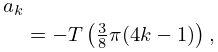
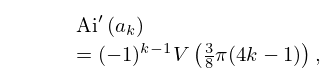
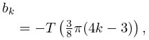
19: 9.9 Zeros

… ►They lie in the sectors and , and are denoted by ${\beta }_k$, ${\beta }_k^{\prime }$, respectively, in the former sector, and by $\overline{{\beta }_k}$, $\overline{{\beta }_k^{\prime }}$, in the conjugate sector, again arranged in ascending order of absolute value (modulus) for $k=1,2,\mathrm{\dots }.$ See §9.3(ii) for visualizations. … ►

9.9.6 $$a_k=-T\left(\frac{3}{8}\pi (4k-1)\right),$$

ⓘ

Symbols:

$\pi$: the ratio of the circumference of a circle to its diameter, $a_k$: $k$th zero of Airy $\mathrm{Ai}$ , $k$: nonnegative integer and $T$: expansion

Source:

Olver (1954, (A 20))

Permalink:

http://dlmf.nist.gov/9.9.E6

Encodings:

pMML, png, TeX

See also:

Annotations for §9.9(iv), §9.9 and Ch.9

►

9.9.7 $${\mathrm{Ai}}^{\prime }\left(a_k\right)={(-1)}^{k-1}V\left(\frac{3}{8}\pi (4k-1)\right),$$

ⓘ

Symbols:

$\mathrm{Ai}\left(z\right)$: Airy function, $\pi$: the ratio of the circumference of a circle to its diameter, $a_k$: $k$th zero of Airy $\mathrm{Ai}$ , $k$: nonnegative integer and $V$: expansion

Source:

Olver (1954, (A 20))

Permalink:

http://dlmf.nist.gov/9.9.E7

Encodings:

pMML, png, TeX

See also:

Annotations for §9.9(iv), §9.9 and Ch.9

… ►

9.9.10 $$b_k=-T\left(\frac{3}{8}\pi (4k-3)\right),$$

ⓘ

Symbols:

$\pi$: the ratio of the circumference of a circle to its diameter, $b_k$: $k$th zero of Airy $\mathrm{Bi}$ , $k$: nonnegative integer and $T$: expansion

Source:

Olver (1954, (A 21))

Permalink:

http://dlmf.nist.gov/9.9.E10

Encodings:

pMML, png, TeX

See also:

Annotations for §9.9(iv), §9.9 and Ch.9

… ►

9.9.21 $$W(t)\sim {\pi }^{-1/2}{t}^{-1/6}\left(1-\frac{7}{96}{t}^{-2}+\frac{1673}{6144}{t}^{-4}-\frac{\mathrm{843\hspace{0.33em}94709}}{\mathrm{265\hspace{0.33em}42080}}{t}^{-6}+\frac{\mathrm{78\hspace{0.33em}02771\hspace{0.33em}35421}}{\mathrm{1\hspace{0.33em}01921\hspace{0.33em}58720}}{t}^{-8}-\frac{\mathrm{20444\hspace{0.33em}90510\hspace{0.33em}51945}}{\mathrm{6\hspace{0.33em}52298\hspace{0.33em}15808}}{t}^{-10}+\mathrm{\cdots }\right).$$

ⓘ

Defines:

$W$: expansion (locally)

Symbols:

$\sim$: Poincaré asymptotic expansion and $\pi$: the ratio of the circumference of a circle to its diameter

Source:

Olver (1954, (A 19))

Permalink:

http://dlmf.nist.gov/9.9.E21

Encodings:

pMML, png, TeX

See also:

Annotations for §9.9(iv), §9.9 and Ch.9

…

20: Bibliography J

… ►

Fonctions de Mathieu et fonctions propres de l’oscillateur relativiste. Ann. Fac. Sci. Toulouse Math. (6) 7 (3), pp. 465–495 (French).

ⓘ

Notes:

Translated title: Mathieu functions and eigenfunctions of the relativistic oscillator.

External Links:

ISSN 0240-2963, Pdf, MathReview (Jean-Michel Ghez), ZentralBlatt

Referenced by:

7th item.

Encodings:

BibTeX

… ►

The birth of the giant component. Random Structures Algorithms 4 (3), pp. 231–358.

ⓘ

Notes:

With an introduction by the editors

External Links:

ISSN 1042-9832, Document, MathReview (Alan M. Frieze), ZentralBlatt

Referenced by:

§16.23(ii), §9.13(ii).

Encodings:

BibTeX

… ►

Numerical calculation of Bessel, Hankel and Airy functions. Computer Physics Communications 183 (3), pp. 506–519.

ⓘ

External Links:

Document, FullText, ZentralBlatt

Referenced by:

§10.19(iii), §10.19(iii).

Encodings:

BibTeX

… ►

Asymptotic formulas for the zeros of the Meixner polynomials. J. Approx. Theory 96 (2), pp. 281–300.

ⓘ

External Links:

ISSN 0021-9045, Document, MathReview (N. Hayek Calil), ZentralBlatt

Referenced by:

§18.24.

Encodings:

BibTeX

… ►

Memoire sur l’itération des fonctions rationnelles. J. Math. Pures Appl. 8 (1), pp. 47–245 (French).

ⓘ

External Links:

FullText, ZentralBlatt

Referenced by:

§3.8(viii).

Encodings:

BibTeX