%E6%97%B6%E6%97%B6%E5%BD%A9%E5%B9%B3%E5%8F%B0,%E6%97%B6%E6%97%B6%E5%BD%A9%E7%8E%A9%E6%B3%95,%E9%87%8D%E5%BA%86%E6%97%B6%E6%97%B6%E5%BD%A9%E6%8A%80%E5%B7%A7,%E6%97%B6%E6%97%B6%E5%BD%A9%E8%A7%84%E5%88%99,%E3%80%90%E6%97%B6%E6%97%B6%E5%BD%A9%E7%BD%91%E5%9D%80%E2%88%B622kk55.com%E3%80%91%E9%87%8D%E5%BA%86%E6%97%B6%E6%97%B6%E5%BD%A9%E5%B9%B3%E5%8F%B0%E6%8E%A8%E8%8D%90,%E6%97%B6%E6%97%B6%E5%BD%A9%E5%AE%98%E7%BD%91,%E9%87%8D%E5%BA%86%E6%97%B6%E6%97%B6%E5%BD%A9%E7%BD%91%E7%AB%99,%E9%87%8D%E5%BA%86%E6%97%B6%E6%97%B6%E5%BD%A9%E8%A7%84%E5%88%99,%E6%97%B6%E6%97%B6%E5%BD%A9%E5%BC%80%E5%A5%96%E7%BB%93%E6%9E%9C,%E6%97%B6%E6%97%B6%E5%BD%A9app%E4%B8%8B%E8%BD%BD,%E3%80%90%E6%97%B6%E6%97%B6%E5%BD%A9%E5%B9%B3%E5%8F%B0%E2%88%B622kk55.com%E3%80%91
(0.036 seconds)
21—30 of 622 matching pages
21: 34.5 Basic Properties: Symbol
…
►
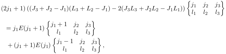
34.5.11
…
►
34.5.13
►For further recursion relations see Varshalovich et al. (1988, §9.6) and Edmonds (1974, pp. 98–99).
…
22: 13.10 Integrals
…
►
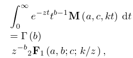
13.10.3
, ,
…
►
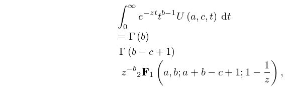
13.10.7
, .
…
►For additional Hankel transforms and also other Bessel transforms see Erdélyi et al. (1954b, §8.18) and Oberhettinger (1972, §§1.16 and 3.4.42–46, 4.4.45–47, 5.94–97).
…
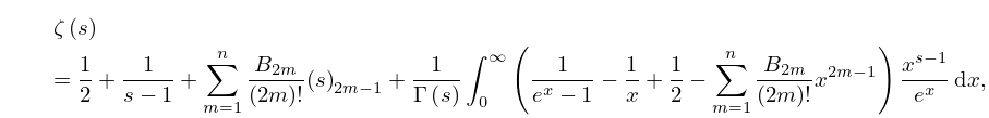
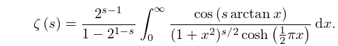
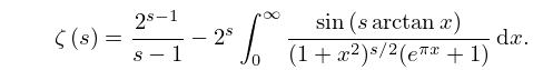
23: 25.5 Integral Representations
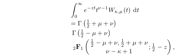
24: 13.23 Integrals
…
►
13.23.1
,
.
…
►
13.23.4
,
,
…
►For additional Hankel transforms and also other Bessel transforms see Erdélyi et al. (1954b, §8.18) and Oberhettinger (1972, §1.16 and 3.4.42–46, 4.4.45–47, 5.94–97).
…
25: 1.9 Calculus of a Complex Variable
…
►Any point whose neighborhoods always contain members and nonmembers of is a boundary point of .
…
►A function is analytic in a domain
if it is analytic at each point of .
…
►at all points of .
…
►Suppose is analytic in a domain and are two arcs in passing through .
…
►for any finite contour in .
…
26: 12.14 The Function
…
►For the modulus functions and see §12.14(x).
…
►Other expansions, involving and , can be obtained from (12.4.3) to (12.4.6) by replacing by and by ; see Miller (1955, p. 80), and also (12.14.15) and (12.14.16).
…
►where is defined in (12.14.5), and (0), , (0), and are real.
or is the modulus and or is the corresponding phase.
…
►For properties of the modulus and phase functions, including differential equations and asymptotic expansions for large , see Miller (1955, pp. 87–88).
…
27: Bibliography O
…
►
Hyperterminants. II.
J. Comput. Appl. Math. 89 (1), pp. 87–95.
…
►
Uniform asymptotic expansions for hypergeometric functions with large parameters. III.
Analysis and Applications (Singapore) 8 (2), pp. 199–210.
…
►
Connection formulas for second-order differential equations with multiple turning points.
SIAM J. Math. Anal. 8 (1), pp. 127–154.
►
Connection formulas for second-order differential equations having an arbitrary number of turning points of arbitrary multiplicities.
SIAM J. Math. Anal. 8 (4), pp. 673–700.
…
►
Whittaker functions with both parameters large: Uniform approximations in terms of parabolic cylinder functions.
Proc. Roy. Soc. Edinburgh Sect. A 86 (3-4), pp. 213–234.
…
28: 26.6 Other Lattice Path Numbers
…
►
Delannoy Number
► is the number of paths from to that are composed of directed line segments of the form , , or . … ► … ►
26.6.4
.
…
►
26.6.10
,
…
29: 10.22 Integrals
…
►In this subsection and denote cylinder functions(§10.2(ii)) of orders and , respectively, not necessarily distinct.
…
►For the hypergeometric function see §15.2(i).
…
►Sufficient conditions for the validity of (10.22.77) are that when , or that and when ; see Titchmarsh (1986a, Theorem 135, Chapter 8) and Akhiezer (1988, p. 62).
…
►For collections of Hankel transforms see Erdélyi et al. (1954b, Chapter 8) and Oberhettinger (1972).
…
►Sufficient conditions for the validity of (10.22.79) are that when , or that and when ; see Titchmarsh (1962a, pp. 88–90).
…
30: Bibliography U
…
►
On the equation
.
Acta Arith. 51 (4), pp. 349–368.
►
On Kelvin’s ship-wave pattern.
J. Fluid Mech. 8 (3), pp. 418–431.
…
►
Integrals with a large parameter: A double complex integral with four nearly coincident saddle-points.
Math. Proc. Cambridge Philos. Soc. 87 (2), pp. 249–273.
►
Integrals with a large parameter: Legendre functions of large degree and fixed order.
Math. Proc. Cambridge Philos. Soc. 95 (2), pp. 367–380.
…
