ultraspherical polynomials

SearchAdvancedHelp

(0.002 seconds)

1—10 of 39 matching pages

1: 18.3 Definitions

§18.3 Definitions

… ►This table also includes the following special cases of Jacobi polynomials: ultraspherical, Chebyshev, and Legendre. ►

Table 18.3.1: Orthogonality properties for classical OP’s: intervals, weight functions, standardizations, leading coefficients, and parameter constraints. …

► ►►►

Name	$p_n(x)$	$(a,b)$	$w(x)$	$h_n$	$k_n$	${\tilde{k}}_n/k_n$	Constraints
…
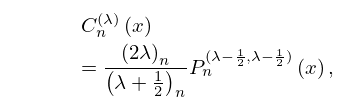
Ultraspherical (Gegenbauer)	$C_n^{(\lambda )}\left(x\right)$	$(-1,1)$	${(1-x^2)}^{\lambda -\frac{1}{2}}$	${\displaystyle \frac{2^{1-2\lambda }\pi \mathrm{\Gamma }\left(n+2\lambda \right)}{(n+\lambda ){\left(\mathrm{\Gamma }\left(\lambda \right)\right)}^{2}n!}}$	${\displaystyle \frac{2^n{\left(\lambda \right)}_n}{n!}}$	$0$	$\lambda >-\frac{1}{2},\lambda \ne 0$
…

►

… ►For explicit power series coefficients up to $n=12$ for these polynomials and for coefficients up to $n=6$ for Jacobi and ultraspherical polynomials see Abramowitz and Stegun (1964, pp. 793–801). …

2: 18.6 Symmetry, Special Values, and Limits to Monomials

… ►For Jacobi, ultraspherical, Chebyshev, Legendre, and Hermite polynomials, see Table 18.6.1. … ►

Table 18.6.1: Classical OP’s: symmetry and special values.

► ►►►

$p_n(x)$	$p_n(-x)$	$p_n(1)$	$p_{2n}(0)$	$p_{2n+1}^{\prime }(0)$
…
$C_n^{(\lambda )}\left(x\right)$	${(-1)}^n{C}_n^{(\lambda )}\left(x\right)$	${\left(2\lambda \right)}_n/n!$	${(-1)}^n{\left(\lambda \right)}_n/n!$	$2{(-1)}^n{\left(\lambda \right)}_{n+1}/n!$
…

►

►

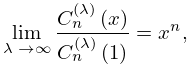
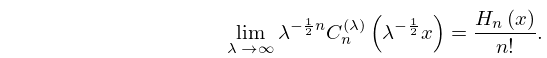
§18.6(ii) Limits to Monomials

… ►

18.6.4 $$\underset{\lambda \to \mathrm{\infty }}{lim}\frac{C_n^{(\lambda )}\left(x\right)}{C_n^{(\lambda )}\left(1\right)}=x^n,$$

ⓘ

Symbols:

$C_n^{(\lambda )}\left(x\right)$: ultraspherical (or Gegenbauer) polynomial, $n$: nonnegative integer and $x$: real variable

Referenced by:

§18.18(iv), §18.6(ii)

Permalink:

http://dlmf.nist.gov/18.6.E4

Encodings:

pMML, png, TeX

See also:

Annotations for §18.6(ii), §18.6 and Ch.18

…

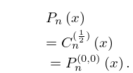
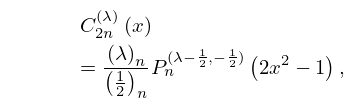
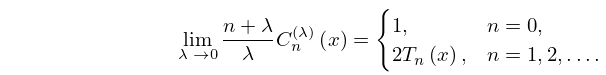
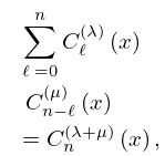
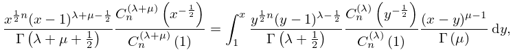
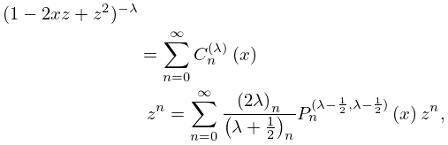
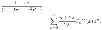
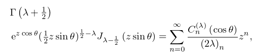
3: 18.7 Interrelations and Limit Relations

… ►

18.7.1 $$C_n^{(\lambda )}\left(x\right)=\frac{{\left(2\lambda \right)}_n}{{\left(\lambda +\frac{1}{2}\right)}_n}{P}_n^{(\lambda -\frac{1}{2},\lambda -\frac{1}{2})}\left(x\right),$$

ⓘ

Symbols:

$P_n^{(\alpha ,\beta )}\left(x\right)$: Jacobi polynomial, ${\left(a\right)}_n$: Pochhammer’s symbol (or shifted factorial), $C_n^{(\lambda )}\left(x\right)$: ultraspherical (or Gegenbauer) polynomial, $n$: nonnegative integer and $x$: real variable

A&S Ref:

22.5.27

Referenced by:

§18.15(ii), §18.7(i), §18.7(ii), §18.7(iii)

Permalink:

http://dlmf.nist.gov/18.7.E1

Encodings:

pMML, png, TeX

See also:

Annotations for §18.7(i), §18.7(i), §18.7 and Ch.18

… ►

18.7.9 $$P_n\left(x\right)=C_n^{(\frac{1}{2})}\left(x\right)=P_n^{(0,0)}\left(x\right).$$

ⓘ

Symbols:

$P_n^{(\alpha ,\beta )}\left(x\right)$: Jacobi polynomial, $P_n\left(x\right)$: Legendre polynomial, $C_n^{(\lambda )}\left(x\right)$: ultraspherical (or Gegenbauer) polynomial, $n$: nonnegative integer and $x$: real variable

A&S Ref:

22.5.35, 22.5.36

Referenced by:

§10.60(iii), §18.18(ii), §18.5(iii)

Permalink:

http://dlmf.nist.gov/18.7.E9

Encodings:

pMML, png, TeX

See also:

Annotations for §18.7(i), §18.7(i), §18.7 and Ch.18

… ►

18.7.15 $$C_{2n}^{(\lambda )}\left(x\right)=\frac{{\left(\lambda \right)}_n}{{\left(\frac{1}{2}\right)}_n}{P}_n^{(\lambda -\frac{1}{2},-\frac{1}{2})}\left(2x^2-1\right),$$

ⓘ

Symbols:

$P_n^{(\alpha ,\beta )}\left(x\right)$: Jacobi polynomial, ${\left(a\right)}_n$: Pochhammer’s symbol (or shifted factorial), $C_n^{(\lambda )}\left(x\right)$: ultraspherical (or Gegenbauer) polynomial, $n$: nonnegative integer and $x$: real variable

A&S Ref:

22.5.25

Referenced by:

§18.7(ii), §18.9(ii)

Permalink:

http://dlmf.nist.gov/18.7.E15

Encodings:

pMML, png, TeX

See also:

Annotations for §18.7(ii), §18.7 and Ch.18

… ►

18.7.24 $$\underset{\lambda \to \mathrm{\infty }}{lim}{\lambda }^{-\frac{1}{2}n}{C}_n^{(\lambda )}\left({\lambda }^{-\frac{1}{2}}x\right)=\frac{H_n\left(x\right)}{n!}.$$

ⓘ

Symbols:

$H_n\left(x\right)$: Hermite polynomial, $!$: factorial (as in $n!$), $C_n^{(\lambda )}\left(x\right)$: ultraspherical (or Gegenbauer) polynomial, $n$: nonnegative integer and $x$: real variable

A&S Ref:

22.15.6

Referenced by:

§18.7(iii)

Permalink:

http://dlmf.nist.gov/18.7.E24

Encodings:

pMML, png, TeX

See also:

Annotations for §18.7(iii), §18.7(iii), §18.7 and Ch.18

… ►

18.7.25

ⓘ

Symbols:

$T_n\left(x\right)$: Chebyshev polynomial of the first kind, $C_n^{(\lambda )}\left(x\right)$: ultraspherical (or Gegenbauer) polynomial, $n$: nonnegative integer and $x$: real variable

Source:

Andrews et al. (1999, (6.4.13))

Referenced by:

§18.7(i), §18.7(iii), Erratum (V1.2.0) for Equation (18.7.25)

Permalink:

http://dlmf.nist.gov/18.7.E25

Encodings:

pMML, png, TeX

Addition (effective with 1.2.0):

We included the case $n=0$.

See also:

Annotations for §18.7(iii), §18.7(iii), §18.7 and Ch.18

…

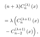
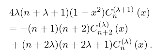
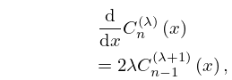
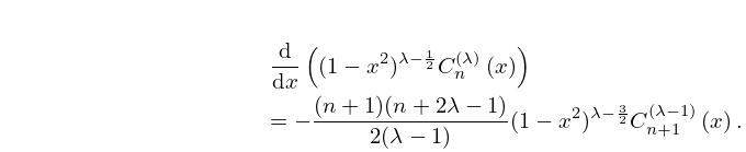
4: 18.9 Recurrence Relations and Derivatives

… ►

18.9.7 $$(n+\lambda )C_n^{(\lambda )}\left(x\right)=\lambda \left(C_n^{(\lambda +1)}\left(x\right)-C_{n-2}^{(\lambda +1)}\left(x\right)\right),$$

ⓘ

Symbols:

$C_n^{(\lambda )}\left(x\right)$: ultraspherical (or Gegenbauer) polynomial, $n$: nonnegative integer and $x$: real variable

Referenced by:

§18.9(ii)

Permalink:

http://dlmf.nist.gov/18.9.E7

Encodings:

pMML, png, TeX

See also:

Annotations for §18.9(ii), §18.9(ii), §18.9 and Ch.18

►

18.9.8 $$4\lambda (n+\lambda +1)(1-x^2)C_n^{(\lambda +1)}\left(x\right)=-(n+1)(n+2)C_{n+2}^{(\lambda )}\left(x\right)+(n+2\lambda )(n+2\lambda +1)C_n^{(\lambda )}\left(x\right).$$

ⓘ

Symbols:

$C_n^{(\lambda )}\left(x\right)$: ultraspherical (or Gegenbauer) polynomial, $n$: nonnegative integer and $x$: real variable

Referenced by:

§18.9(ii)

Permalink:

http://dlmf.nist.gov/18.9.E8

Encodings:

pMML, png, TeX

See also:

Annotations for §18.9(ii), §18.9(ii), §18.9 and Ch.18

… ►

Ultraspherical

►

18.9.19 $$\frac{d}{dx}{C}_n^{(\lambda )}\left(x\right)=2\lambda C_{n-1}^{(\lambda +1)}\left(x\right),$$

ⓘ

Symbols:

$\frac{df}{dx}$: derivative of $f$ with respect to $x$ , $C_n^{(\lambda )}\left(x\right)$: ultraspherical (or Gegenbauer) polynomial, $n$: nonnegative integer and $x$: real variable

Referenced by:

§1.10(xi), §18.17(i), §18.9(iii)

Permalink:

http://dlmf.nist.gov/18.9.E19

Encodings:

pMML, png, TeX

See also:

Annotations for §18.9(iii), §18.9(iii), §18.9 and Ch.18

►

18.9.20 $$\frac{d}{dx}\left({(1-x^2)}^{\lambda -\frac{1}{2}}{C}_n^{(\lambda )}\left(x\right)\right)=-\frac{(n+1)(n+2\lambda -1)}{2(\lambda -1)}{(1-x^2)}^{\lambda -\frac{3}{2}}{C}_{n+1}^{(\lambda -1)}\left(x\right).$$

ⓘ

Symbols:

$\frac{df}{dx}$: derivative of $f$ with respect to $x$ , $C_n^{(\lambda )}\left(x\right)$: ultraspherical (or Gegenbauer) polynomial, $n$: nonnegative integer and $x$: real variable

Referenced by:

§18.9(iii)

Permalink:

http://dlmf.nist.gov/18.9.E20

Encodings:

pMML, png, TeX

See also:

Annotations for §18.9(iii), §18.9(iii), §18.9 and Ch.18

…

5: 18.1 Notation

… ►

Ultraspherical (or Gegenbauer): $C_n^{(\lambda )}\left(x\right)$.

… ►

Continuous $q$-Ultraspherical: $C_n(x;\beta |q)$.

… ►In Szegő (1975, §4.7) the ultraspherical polynomials $C_n^{(\lambda )}\left(x\right)$ are denoted by $P_n^{(\lambda )}(x)$. The ultraspherical polynomials will not be considered for $\lambda =0$. They are defined in the literature by $C_0^{(0)}\left(x\right)=1$ and …

6: 18.10 Integral Representations

… ►

Ultraspherical

►

18.10.1 $$\frac{P_n^{(\alpha ,\alpha )}\left(\cos \theta \right)}{P_n^{(\alpha ,\alpha )}\left(1\right)}=\frac{C_n^{(\alpha +\frac{1}{2})}\left(\cos \theta \right)}{C_n^{(\alpha +\frac{1}{2})}\left(1\right)}=\frac{2^{\alpha +\frac{1}{2}}\mathrm{\Gamma }\left(\alpha +1\right)}{{\pi }^{\frac{1}{2}}\mathrm{\Gamma }\left(\alpha +\frac{1}{2}\right)}{(\sin \theta )}^{-2\alpha }{\int }_0^{\theta }\frac{\cos \left((n+\alpha +\frac{1}{2})\varphi \right)}{{(\cos \varphi -\cos \theta )}^{-\alpha +\frac{1}{2}}}d\varphi ,$$ , $\alpha >-\frac{1}{2}$.

ⓘ

Symbols:

$\mathrm{\Gamma }\left(z\right)$: gamma function, $P_n^{(\alpha ,\beta )}\left(x\right)$: Jacobi polynomial, $\pi$: the ratio of the circumference of a circle to its diameter, $\cos z$: cosine function, $dx$: differential of $x$ , $\int$: integral, $\sin z$: sine function, $C_n^{(\lambda )}\left(x\right)$: ultraspherical (or Gegenbauer) polynomial and $n$: nonnegative integer

A&S Ref:

22.10.11

Referenced by:

§18.10(i), §18.10(i)

Permalink:

http://dlmf.nist.gov/18.10.E1

Encodings:

pMML, png, TeX

See also:

Annotations for §18.10(i), §18.10(i), §18.10 and Ch.18

… ►

Ultraspherical

►

18.10.4 $$\frac{P_n^{(\alpha ,\alpha )}\left(\cos \theta \right)}{P_n^{(\alpha ,\alpha )}\left(1\right)}=\frac{C_n^{(\alpha +\frac{1}{2})}\left(\cos \theta \right)}{C_n^{(\alpha +\frac{1}{2})}\left(1\right)}=\frac{\mathrm{\Gamma }\left(\alpha +1\right)}{{\pi }^{\frac{1}{2}}\mathrm{\Gamma }(\alpha +\frac{1}{2})}{\int }_0^{\pi }{(\cos \theta +i\sin \theta \cos \varphi )}^n{(\sin \varphi )}^{2\alpha }d\varphi ,$$ $\alpha >-\frac{1}{2}$.

ⓘ

Symbols:

$\mathrm{\Gamma }\left(z\right)$: gamma function, $P_n^{(\alpha ,\beta )}\left(x\right)$: Jacobi polynomial, $\pi$: the ratio of the circumference of a circle to its diameter, $\cos z$: cosine function, $dx$: differential of $x$ , $\int$: integral, $\sin z$: sine function, $C_n^{(\lambda )}\left(x\right)$: ultraspherical (or Gegenbauer) polynomial and $n$: nonnegative integer

A&S Ref:

22.10.10

Referenced by:

§18.10(ii)

Permalink:

http://dlmf.nist.gov/18.10.E4

Encodings:

pMML, png, TeX

See also:

Annotations for §18.10(ii), §18.10(ii), §18.10 and Ch.18

… ►

Table 18.10.1: Classical OP’s: contour integral representations (18.10.8).

► ►►►

$p_n(x)$	$g_0(x)$	$g_1(z,x)$	$g_2(z,x)$	$c$	Conditions
…
$C_n^{(\lambda )}\left(x\right)$	$1$	$z^{-1}$	${(1-2xz+z^2)}^{-\lambda }$	$0$	${\mathrm{e}}^{\pm \mathrm{i}\theta }$ outside $C$ (where $x=\cos \theta$).
…

►

…

7: 37.4 Disk with Weight Function ${\left(1-x^2-y^2\right)}^{\alpha }$

… ►

37.4.5 $$C_{k,n}^{(\alpha +\frac{1}{2})}(x,y)=C_{n-k}^{(\alpha +k+1)}\left(x\right){(1-x^2)}^{\frac{1}{2}k}{C}_k^{(\alpha +\frac{1}{2})}\left(\frac{y}{\sqrt{1-x^2}}\right).$$

ⓘ

Defines:

$C_{k,n}^{(\alpha +\frac{1}{2})}(x,y)$: two-variable ultraspherical polynomial on the disk

Symbols:

$C_n^{(\lambda )}\left(x\right)$: ultraspherical (or Gegenbauer) polynomial, $k$: nonnegative integer, $n$: nonnegative integer, $x$: real variable, $y$: real variable and $\alpha$: real parameter

Source:

Dunkl and Xu (2014, (2.3.1)); The mentioned value of the constant in (37.4.4) follows by (18.7.1).

Referenced by:

§37.15(ii), (37.4.29), §37.4(ii), §37.4(iii), §37.4(vi)

Permalink:

http://dlmf.nist.gov/37.4.E5

Encodings:

pMML, png, TeX

See also:

Annotations for §37.4(ii), §37.4, Part 37.II and Ch.37

… ►

37.4.6 $${⟨C_{k,n}^{(\alpha +\frac{1}{2})},C_{j,m}^{(\alpha +\frac{1}{2})}⟩}_{\alpha }=h_{k,n}^{(\alpha +\frac{1}{2})}{\delta }_{n,m}{\delta }_{k,j},$$

ⓘ

Symbols:

${\delta }_{j,k}$: Kronecker delta, $C_{k,n}^{(\alpha +\frac{1}{2})}(x,y)$: two-variable ultraspherical polynomial on the disk, $j$: nonnegative integer, $k$: nonnegative integer, $m$: nonnegative integer, $n$: nonnegative integer, $\alpha$: real parameter, ${⟨f,g⟩}_{\alpha }$: inner product on disk and $h_{k,n}^{(\alpha +\frac{1}{2})}$: orthogonality norm for two-variable ultraspherical polynomial on $𝔻$

Permalink:

http://dlmf.nist.gov/37.4.E6

Encodings:

pMML, png, TeX

See also:

Annotations for §37.4(ii), §37.4, Part 37.II and Ch.37

… ►There is also an orthogonal basis of ${𝒱}_n^{\alpha }$ consisting of polynomials $C_{k,n}^{(\alpha +\frac{1}{2})}(y,x)$ ($k=0,1,\mathrm{\dots },n$). … ►For $\alpha =0$, by (18.7.4), $C_n^{(1)}=U_n$, the Chebyshev polynomial of the second kind. … ►

37.4.29 $$[(1-x^2-y^2)D_{yy}-2(\alpha +1)y{D}_y]C_{k,n}^{(\alpha +\frac{1}{2})}(x,y)=-k(k+2\alpha +1)C_{k,n}^{(\alpha +\frac{1}{2})}(x,y),$$

ⓘ

Symbols:

$\frac{df}{dx}$: derivative of $f$ with respect to $x$ , $C_{k,n}^{(\alpha +\frac{1}{2})}(x,y)$: two-variable ultraspherical polynomial on the disk, $k$: nonnegative integer, $n$: nonnegative integer, $z$: complex number, $x$: real variable, $y$: real variable and $\alpha$: real parameter

Proof sketch:

From (37.4.5) and Table 18.8.1 we get $\left[(1-z^2)D_{zz}-2(\alpha +1)D_z+k(k+2\alpha +1)\right]C_{k,n}^{(\alpha +\frac{1}{2})}(x,z\sqrt{1-x^2})=0$.

Permalink:

http://dlmf.nist.gov/37.4.E29

Encodings:

pMML, png, TeX

See also:

Annotations for §37.4(vi), §37.4, Part 37.II and Ch.37

…

8: 37.11 Spherical Harmonics

… ►

37.11.15 $$Y(\xi )=\mathrm{const}.P_n^{(\frac{1}{2}(d-3),\frac{1}{2}(d-3))}\left({\xi }_1\right)=\mathrm{const}.C_n^{(\frac{1}{2}(d-2))}\left({\xi }_1\right),$$ $\xi =({\xi }_1,\mathrm{\dots },{\xi }_d)\in {𝕊}^{d-1}$.

ⓘ

Symbols:

$P_n^{(\alpha ,\beta )}\left(x\right)$: Jacobi polynomial, $\in$: element of, $C_n^{(\lambda )}\left(x\right)$: ultraspherical (or Gegenbauer) polynomial, $n$: nonnegative integer, $d$: positive integer, usually $\ge 2$ and ${𝕊}^{d-1}$: unit sphere of dimension $d-1$

Permalink:

http://dlmf.nist.gov/37.11.E15

Encodings:

pMML, png, TeX

See also:

Annotations for §37.11(i), §37.11(i), §37.11, Part 37.III and Ch.37

… ►

37.11.18 $$Y_{𝐧}(\xi )={\mathrm{e}}^{\pm \mathrm{i}{n}_{d-1}{\theta }_{d-1}}\prod _{j=1}^{d-2}{C}_{n_j-n_{j+1}}^{(\frac{1}{2}(d-j-1)+n_{j+1})}\left(\cos {\theta }_j\right){\left(\sin {\theta }_j\right)}^{n_{j+1}},$$ $n=n_1\ge n_2\ge \mathrm{\cdots }\ge n_{d-1}\ge 0$

ⓘ

Symbols:

$\cos z$: cosine function, $\mathrm{e}$: base of natural logarithm, $\mathrm{i}$: imaginary unit, $\sin z$: sine function, $C_n^{(\lambda )}\left(x\right)$: ultraspherical (or Gegenbauer) polynomial, $j$: nonnegative integer, $n$: nonnegative integer and $d$: positive integer, usually $\ge 2$

Proof sketch:

Iterate (37.11.16)

Referenced by:

§37.11(iii), §37.11(iii), §37.12(i)

Permalink:

http://dlmf.nist.gov/37.11.E18

Encodings:

pMML, png, TeX

See also:

Annotations for §37.11(i), §37.11(i), §37.11, Part 37.III and Ch.37

… ►

37.11.27 $${𝐑}_n(\xi ,\eta )=\sum _{j=1}^{N_n^d}{Y}_j(\xi )\overline{Y_j(\eta )}=N_n^d\frac{C_n^{(\frac{1}{2}(d-2))}\left(⟨\xi ,\eta ⟩\right)}{C_n^{(\frac{1}{2}(d-2))}\left(1\right)}=Z_n^{(\frac{1}{2}(d-2))}(⟨\xi ,\eta ⟩),$$ $\xi ,\eta \in {𝕊}^{d-1}$.

ⓘ

Symbols:

$\overline{z}$: complex conjugate, $\in$: element of, $⟨𝐮,𝐯⟩$: inner product over vectors, $C_n^{(\lambda )}\left(x\right)$: ultraspherical (or Gegenbauer) polynomial, $j$: nonnegative integer, $n$: nonnegative integer, $d$: positive integer, usually $\ge 2$ , ${𝕊}^{d-1}$: unit sphere of dimension $d-1$ and ${𝐑}_n$: reproducing kernel

Proved:

Dai and Xu (2013, (1.2.7), (1.2.8))(proved)

Referenced by:

§37.11(iii), §37.11(iii)

Permalink:

http://dlmf.nist.gov/37.11.E27

Encodings:

pMML, png, TeX

See also:

Annotations for §37.11(iii), §37.11(iii), §37.11, Part 37.III and Ch.37

… ►

37.11.28 $$Z_n^{(\lambda )}(x)=\frac{{\int }_{-1}^1{\left(1-t^2\right)}^{\lambda -\frac{1}{2}}dt}{{\int }_{-1}^1{C_n^{(\lambda )}\left(t\right)}^2{\left(1-t^2\right)}^{\lambda -\frac{1}{2}}dt}{C}_n^{(\lambda )}\left(x\right)C_n^{(\lambda )}\left(1\right)=\frac{n+\lambda }{\lambda }{C}_n^{(\lambda )}\left(x\right).$$

ⓘ

Symbols:

$dx$: differential of $x$ , $\int$: integral, $C_n^{(\lambda )}\left(x\right)$: ultraspherical (or Gegenbauer) polynomial, $n$: nonnegative integer and $x$: real variable

Referenced by:

§37.12(ii), §37.14(v), §37.15(vi), §37.18(ii)

Permalink:

http://dlmf.nist.gov/37.11.E28

Encodings:

pMML, png, TeX

See also:

Annotations for §37.11(iii), §37.11(iii), §37.11, Part 37.III and Ch.37

… ► …

9: 18.18 Sums

… ►

Ultraspherical

… ►

Ultraspherical

… ►

Ultraspherical

►

18.18.29 $$\sum _{\mathrm{\ell }=0}^n{C}_{\mathrm{\ell }}^{(\lambda )}\left(x\right)C_{n-\mathrm{\ell }}^{(\mu )}\left(x\right)=C_n^{(\lambda +\mu )}\left(x\right),$$

ⓘ

Symbols:

$C_n^{(\lambda )}\left(x\right)$: ultraspherical (or Gegenbauer) polynomial, $\mathrm{\ell }$: nonnegative integer, $n$: nonnegative integer and $x$: real variable

Referenced by:

§18.18(viii)

Permalink:

http://dlmf.nist.gov/18.18.E29

Encodings:

pMML, png, TeX

See also:

Annotations for §18.18(viii), §18.18(viii), §18.18 and Ch.18

►

18.18.30 $$\sum _{\mathrm{\ell }=0}^n\frac{\mathrm{\ell }+2\lambda }{2\lambda }{C}_{\mathrm{\ell }}^{(\lambda )}\left(x\right)x^{n-\mathrm{\ell }}=C_n^{(\lambda +1)}\left(x\right).$$

ⓘ

Symbols:

$C_n^{(\lambda )}\left(x\right)$: ultraspherical (or Gegenbauer) polynomial, $\mathrm{\ell }$: nonnegative integer, $n$: nonnegative integer and $x$: real variable

Referenced by:

§18.18(viii)

Permalink:

http://dlmf.nist.gov/18.18.E30

Encodings:

pMML, png, TeX

See also:

Annotations for §18.18(viii), §18.18(viii), §18.18 and Ch.18

…

10: 18.17 Integrals

… ►

Ultraspherical

… ►

Ultraspherical

… ►

18.17.13 $$\frac{x^{\frac{1}{2}n}{(x-1)}^{\lambda +\mu -\frac{1}{2}}}{\mathrm{\Gamma }\left(\lambda +\mu +\frac{1}{2}\right)}\frac{C_n^{(\lambda +\mu )}\left(x^{-\frac{1}{2}}\right)}{C_n^{(\lambda +\mu )}\left(1\right)}={\int }_1^x\frac{y^{\frac{1}{2}n}{(y-1)}^{\lambda -\frac{1}{2}}}{\mathrm{\Gamma }\left(\lambda +\frac{1}{2}\right)}\frac{C_n^{(\lambda )}\left(y^{-\frac{1}{2}}\right)}{C_n^{(\lambda )}\left(1\right)}\frac{{(x-y)}^{\mu -1}}{\mathrm{\Gamma }\left(\mu \right)}dy,$$ $\mu >0$, $x>1$.

ⓘ

Symbols:

$\mathrm{\Gamma }\left(z\right)$: gamma function, $dx$: differential of $x$ , $\int$: integral, $C_n^{(\lambda )}\left(x\right)$: ultraspherical (or Gegenbauer) polynomial, $y$: real variable, $n$: nonnegative integer and $x$: real variable

Referenced by:

§1.15(vi), §18.17(iv)

Permalink:

http://dlmf.nist.gov/18.17.E13

Encodings:

pMML, png, TeX

See also:

Annotations for §18.17(iv), §18.17(iv), §18.17 and Ch.18

… ►

Ultraspherical

… ►

Ultraspherical

…