Jacobi polynomials

SearchAdvancedHelp

(0.002 seconds)

1—10 of 85 matching pages

1: 18.3 Definitions

§18.3 Definitions

… ►

Table 18.3.1: Orthogonality properties for classical OP’s: intervals, weight functions, standardizations, leading coefficients, and parameter constraints. …

► ►►►

Name	$p_n(x)$	$(a,b)$	$w(x)$	$h_n$	$k_n$	${\tilde{k}}_n/k_n$	Constraints
Jacobi	$P_n^{(\alpha ,\beta )}\left(x\right)$	$(-1,1)$	${(1-x)}^{\alpha }{(1+x)}^{\beta }$	${𝒜}_n$	${\displaystyle \frac{{\left(n+\alpha +\beta +1\right)}_n}{2^{n}n!}}$	${\displaystyle \frac{n(\alpha -\beta )}{2n+\alpha +\beta }}$	$\alpha ,\beta >-1$
…

►

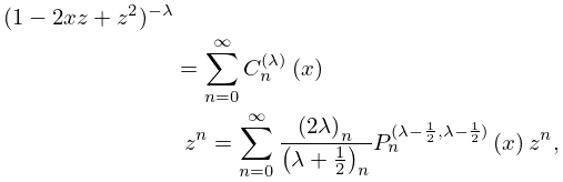
►For expressions of ultraspherical, Chebyshev, and Legendre polynomials in terms of Jacobi polynomials, see §18.7(i). … ►For $-1-\beta >\alpha >-1$ a finite system of Jacobi polynomials $P_n^{(\alpha ,\beta )}\left(x\right)$ is orthogonal on $(1,\mathrm{\infty })$ with weight function $w(x)={(x-1)}^{\alpha }{(x+1)}^{\beta }$. For $\nu \in ℝ$ and $N>-\frac{1}{2}$ a finite system of Jacobi polynomials $P_n^{(-N-1+\mathrm{i}\nu ,-N-1-\mathrm{i}\nu )}\left(\mathrm{i}x\right)$ (called pseudo Jacobi polynomials or Routh–Romanovski polynomials) is orthogonal on $(-\mathrm{\infty },\mathrm{\infty })$ with $w(x)={\left(1+x^2\right)}^{-N-1}{\mathrm{e}}^{2\nu \arctan x}$. …

2: 18.7 Interrelations and Limit Relations

… ►

18.7.3 $$T_n\left(x\right)=P_n^{(-\frac{1}{2},-\frac{1}{2})}\left(x\right)/P_n^{(-\frac{1}{2},-\frac{1}{2})}\left(1\right),$$

ⓘ

Symbols:

$T_n\left(x\right)$: Chebyshev polynomial of the first kind, $P_n^{(\alpha ,\beta )}\left(x\right)$: Jacobi polynomial, $n$: nonnegative integer and $x$: real variable

A&S Ref:

22.3.15, 22.5.31

Referenced by:

§18.17(viii), §18.18(i), §18.5(iii), §18.7(i), §18.7(i), §18.7(ii)

Permalink:

http://dlmf.nist.gov/18.7.E3

Encodings:

pMML, png, TeX

See also:

Annotations for §18.7(i), §18.7(i), §18.7 and Ch.18

►

18.7.4 $$U_n\left(x\right)=C_n^{(1)}\left(x\right)=(n+1)P_n^{(\frac{1}{2},\frac{1}{2})}\left(x\right)/P_n^{(\frac{1}{2},\frac{1}{2})}\left(1\right),$$

ⓘ

Symbols:

$U_n\left(x\right)$: Chebyshev polynomial of the second kind, $P_n^{(\alpha ,\beta )}\left(x\right)$: Jacobi polynomial, $C_n^{(\lambda )}\left(x\right)$: ultraspherical (or Gegenbauer) polynomial, $n$: nonnegative integer and $x$: real variable

A&S Ref:

22.3.16, 22.5.32

Referenced by:

§18.12, §18.3, §18.7(i), §18.7(ii)

Permalink:

http://dlmf.nist.gov/18.7.E4

Encodings:

pMML, png, TeX

See also:

Annotations for §18.7(i), §18.7(i), §18.7 and Ch.18

… ►

18.7.13 $$\frac{P_{2n}^{(\alpha ,\alpha )}\left(x\right)}{P_{2n}^{(\alpha ,\alpha )}\left(1\right)}=\frac{P_n^{(\alpha ,-\frac{1}{2})}\left(2x^2-1\right)}{P_n^{(\alpha ,-\frac{1}{2})}\left(1\right)},$$

ⓘ

Symbols:

$P_n^{(\alpha ,\beta )}\left(x\right)$: Jacobi polynomial, $n$: nonnegative integer and $x$: real variable

Referenced by:

§18.7(ii), §18.7(ii)

Permalink:

http://dlmf.nist.gov/18.7.E13

Encodings:

pMML, png, TeX

See also:

Annotations for §18.7(ii), §18.7 and Ch.18

►

18.7.14 $$\frac{P_{2n+1}^{(\alpha ,\alpha )}\left(x\right)}{P_{2n+1}^{(\alpha ,\alpha )}\left(1\right)}=\frac{x{P}_n^{(\alpha ,\frac{1}{2})}\left(2x^2-1\right)}{P_n^{(\alpha ,\frac{1}{2})}\left(1\right)}.$$

ⓘ

Symbols:

$P_n^{(\alpha ,\beta )}\left(x\right)$: Jacobi polynomial, $n$: nonnegative integer and $x$: real variable

Referenced by:

§18.7(ii)

Permalink:

http://dlmf.nist.gov/18.7.E14

Encodings:

pMML, png, TeX

See also:

Annotations for §18.7(ii), §18.7 and Ch.18

… ►

18.7.23 $$\underset{\alpha \to \mathrm{\infty }}{lim}{\alpha }^{-\frac{1}{2}n}{P}_n^{(\alpha ,\alpha )}\left({\alpha }^{-\frac{1}{2}}x\right)=\frac{H_n\left(x\right)}{2^{n}n!}.$$

ⓘ

Symbols:

$H_n\left(x\right)$: Hermite polynomial, $P_n^{(\alpha ,\beta )}\left(x\right)$: Jacobi polynomial, $!$: factorial (as in $n!$), $n$: nonnegative integer and $x$: real variable

Referenced by:

§18.10(ii), §18.7(iii)

Permalink:

http://dlmf.nist.gov/18.7.E23

Encodings:

pMML, png, TeX

See also:

Annotations for §18.7(iii), §18.7(iii), §18.7 and Ch.18

…

3: 18.14 Inequalities

… ►

Jacobi

… ►

Jacobi

►Let $R_n(x)=P_n^{(\alpha ,\beta )}\left(x\right)/P_n^{(\alpha ,\beta )}\left(1\right)$. … ►

Jacobi

… ►

Szegő–Szász Inequality

…

4: 37.3 Triangular Region with Weight Function

… ►Jacobi polynomials on the triangle … ►

37.3.7

ⓘ

Symbols:

: two-variable Jacobi polynomial on the triangle, $n$: nonnegative integer, $k$: nonnegative integer, $x$: real variable, $y$: real variable, : real parameter ($>-1$), : real parameter ($>-1$) and : real parameter ($>-1$)

Proof sketch:

Apply the symmetry in the second row of Table 18.6.1 to the second Jacobi polynomial in (37.3.3).

Referenced by:

(37.3.28)

Permalink:

http://dlmf.nist.gov/37.3.E7

Encodings:

pMML, png, TeX

See also:

Annotations for §37.3(ii), §37.3 and Ch.37

… ►

37.3.8

ⓘ

Defines:

: two-variable $Q$-Jacobi polynomial on the triangle

Symbols:

$P_n^{(\alpha ,\beta )}\left(x\right)$: Jacobi polynomial, : two-variable Jacobi polynomial on the triangle, $n$: nonnegative integer, $k$: nonnegative integer, $Q$: polynomial of two variables, $x$: real variable, $y$: real variable, : real parameter ($>-1$), : real parameter ($>-1$) and : real parameter ($>-1$)

Proved:

Iliev and Xu (2017, §4)(proved)

Referenced by:

§37.5(iii)

Permalink:

http://dlmf.nist.gov/37.3.E8

Encodings:

pMML, png, TeX

See also:

Annotations for §37.3(ii), §37.3 and Ch.37

►

37.3.9

ⓘ

Defines:

: two-variable $R$-Jacobi polynomial on the triangle

Symbols:

$P_n^{(\alpha ,\beta )}\left(x\right)$: Jacobi polynomial, : two-variable Jacobi polynomial on the triangle, $n$: nonnegative integer, $k$: nonnegative integer, $x$: real variable, $y$: real variable, : real parameter ($>-1$), : real parameter ($>-1$) and : real parameter ($>-1$)

Proved:

Iliev and Xu (2017, §4)(proved)

Referenced by:

§37.4(vii), §37.5(iii), §37.7(iv)

Permalink:

http://dlmf.nist.gov/37.3.E9

Encodings:

pMML, png, TeX

See also:

Annotations for §37.3(ii), §37.3 and Ch.37

… ►The first expression for in (37.3.12) is an analogue of the Rodrigues formulas in §18.5(ii). …

5: 18.6 Symmetry, Special Values, and Limits to Monomials

… ►

Table 18.6.1: Classical OP’s: symmetry and special values.

► ►►►►

$p_n(x)$	$p_n(-x)$	$p_n(1)$	$p_{2n}(0)$	$p_{2n+1}^{\prime }(0)$
$P_n^{(\alpha ,\beta )}\left(x\right)$	${(-1)}^n{P}_n^{(\beta ,\alpha )}\left(x\right)$	${\left(\alpha +1\right)}_n/n!$
$P_n^{(\alpha ,\alpha )}\left(x\right)$	${(-1)}^n{P}_n^{(\alpha ,\alpha )}\left(x\right)$	${\left(\alpha +1\right)}_n/n!$	${(-\frac{1}{4})}^n{\left(n+\alpha +1\right)}_n/n!$	${(-\frac{1}{4})}^n{\left(n+\alpha +1\right)}_{n+1}/n!$
…

►

►

§18.6(ii) Limits to Monomials

►

18.6.2 $$\underset{\alpha \to \mathrm{\infty }}{lim}\frac{P_n^{(\alpha ,\beta )}\left(x\right)}{P_n^{(\alpha ,\beta )}\left(1\right)}={\left(\frac{1+x}{2}\right)}^n,$$

ⓘ

Symbols:

$P_n^{(\alpha ,\beta )}\left(x\right)$: Jacobi polynomial, $n$: nonnegative integer and $x$: real variable

Referenced by:

§18.6(ii)

Permalink:

http://dlmf.nist.gov/18.6.E2

Encodings:

pMML, png, TeX

See also:

Annotations for §18.6(ii), §18.6 and Ch.18

►

18.6.3 $$\underset{\beta \to \mathrm{\infty }}{lim}\frac{P_n^{(\alpha ,\beta )}\left(x\right)}{P_n^{(\alpha ,\beta )}\left(-1\right)}={\left(\frac{1-x}{2}\right)}^n,$$

ⓘ

Symbols:

$P_n^{(\alpha ,\beta )}\left(x\right)$: Jacobi polynomial, $n$: nonnegative integer and $x$: real variable

Referenced by:

§18.6(ii)

Permalink:

http://dlmf.nist.gov/18.6.E3

Encodings:

pMML, png, TeX

See also:

Annotations for §18.6(ii), §18.6 and Ch.18

…

6: 18.4 Graphics

… ►

►►

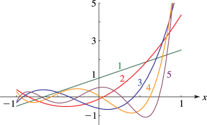
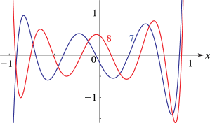
Figure 18.4.1: Jacobi polynomials $P_n^{(1.5,-0.5)}\left(x\right)$, $n=1,2,3,4,5$. Magnify

►

►►

Figure 18.4.2: Jacobi polynomials $P_n^{(1.25,0.75)}\left(x\right)$, $n=7,8$. This illustrates inequalities for extrema of a Jacobi polynomial; see (18.14.16). … Magnify

…

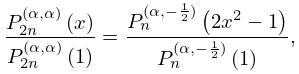
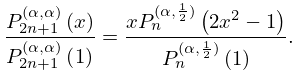
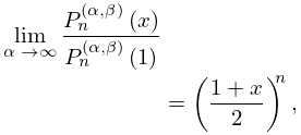
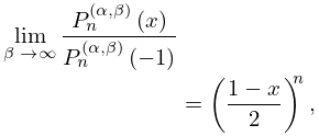
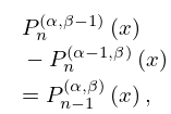
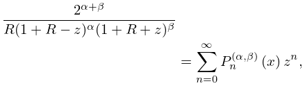
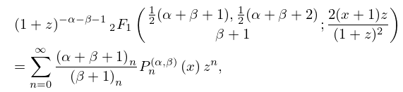
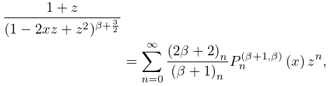
7: 18.9 Recurrence Relations and Derivatives

… ►For $p_n(x)=P_n^{(\alpha ,\beta )}\left(x\right)$, … ►For $p_n(x)=P_n^{(\alpha ,\beta )}\left(x\right)$, … ►

18.9.3 $$P_n^{(\alpha ,\beta -1)}\left(x\right)-P_n^{(\alpha -1,\beta )}\left(x\right)=P_{n-1}^{(\alpha ,\beta )}\left(x\right),$$

ⓘ

Symbols:

$P_n^{(\alpha ,\beta )}\left(x\right)$: Jacobi polynomial, $n$: nonnegative integer and $x$: real variable

A&S Ref:

22.7.20

Referenced by:

§18.9(ii)

Permalink:

http://dlmf.nist.gov/18.9.E3

Encodings:

pMML, png, TeX

See also:

Annotations for §18.9(ii), §18.9(ii), §18.9 and Ch.18

►

18.9.4 $$(1-x)P_n^{(\alpha +1,\beta )}\left(x\right)+(1+x)P_n^{(\alpha ,\beta +1)}\left(x\right)=2P_n^{(\alpha ,\beta )}\left(x\right),$$

ⓘ

Symbols:

$P_n^{(\alpha ,\beta )}\left(x\right)$: Jacobi polynomial, $n$: nonnegative integer and $x$: real variable

A&S Ref:

22.7.17

Permalink:

http://dlmf.nist.gov/18.9.E4

Encodings:

pMML, png, TeX

See also:

Annotations for §18.9(ii), §18.9(ii), §18.9 and Ch.18

… ►

Jacobi

…

8: 37.4 Disk with Weight Function ${\left(1-x^2-y^2\right)}^{\alpha }$

… ►

37.4.4 $$\mathrm{const}.P_{n-k}^{(\alpha +k+\frac{1}{2},\alpha +k+\frac{1}{2})}\left(x\right){(1-x^2)}^{\frac{1}{2}k}{P}_k^{(\alpha ,\alpha )}\left(\frac{y}{\sqrt{1-x^2}}\right)$$

ⓘ

Symbols:

$P_n^{(\alpha ,\beta )}\left(x\right)$: Jacobi polynomial, $n$: nonnegative integer, $k$: nonnegative integer, $x$: real variable, $y$: real variable and $\alpha$: real parameter

Referenced by:

(37.4.5), §37.4(ii), §37.4(vii), §37.7(ii)

Permalink:

http://dlmf.nist.gov/37.4.E4

Encodings:

pMML, png, TeX

See also:

Annotations for §37.4(ii), §37.4 and Ch.37

… ►For Jacobi polynomial $P_n^{(\alpha ,\beta )}\left(x\right)$ in one variable, given in Table 18.3.1, we will use the standardization ►

$R_n^{(\alpha ,\beta )}\left(x\right)={\displaystyle \frac{P_n^{(\alpha ,\beta )}\left(x\right)}{P_n^{(\alpha ,\beta )}\left(1\right)}},$

►

$R_n^{(\alpha ,\beta )}\left(1\right)=1.$

►Then, for $k\in {\mathbb{N}}_0$, the polynomials $R_n^{(\alpha ,k)}\left(2x-1\right)$ are orthogonal on $(0,1)$ with weight function ${(1-x)}^{\alpha }{x}^k$. …

9: 18.10 Integral Representations

… ►

18.10.1 $$\frac{P_n^{(\alpha ,\alpha )}\left(\cos \theta \right)}{P_n^{(\alpha ,\alpha )}\left(1\right)}=\frac{C_n^{(\alpha +\frac{1}{2})}\left(\cos \theta \right)}{C_n^{(\alpha +\frac{1}{2})}\left(1\right)}=\frac{2^{\alpha +\frac{1}{2}}\mathrm{\Gamma }\left(\alpha +1\right)}{{\pi }^{\frac{1}{2}}\mathrm{\Gamma }\left(\alpha +\frac{1}{2}\right)}{(\sin \theta )}^{-2\alpha }{\int }_0^{\theta }\frac{\cos \left((n+\alpha +\frac{1}{2})\varphi \right)}{{(\cos \varphi -\cos \theta )}^{-\alpha +\frac{1}{2}}}d\varphi ,$$ , $\alpha >-\frac{1}{2}$.

ⓘ

Symbols:

$\mathrm{\Gamma }\left(z\right)$: gamma function, $P_n^{(\alpha ,\beta )}\left(x\right)$: Jacobi polynomial, $\pi$: the ratio of the circumference of a circle to its diameter, $\cos z$: cosine function, $dx$: differential of $x$ , $\int$: integral, $\sin z$: sine function, $C_n^{(\lambda )}\left(x\right)$: ultraspherical (or Gegenbauer) polynomial and $n$: nonnegative integer

A&S Ref:

22.10.11

Referenced by:

§18.10(i), §18.10(i)

Permalink:

http://dlmf.nist.gov/18.10.E1

Encodings:

pMML, png, TeX

See also:

Annotations for §18.10(i), §18.10(i), §18.10 and Ch.18

… ►Generalizations of (18.10.1) for $P_n^{(\alpha ,\beta )}$ are given in Gasper (1975, (6),(8)) and Koornwinder (1975a, (5.7),(5.8)). … ►

Jacobi

… ►

18.10.4 $$\frac{P_n^{(\alpha ,\alpha )}\left(\cos \theta \right)}{P_n^{(\alpha ,\alpha )}\left(1\right)}=\frac{C_n^{(\alpha +\frac{1}{2})}\left(\cos \theta \right)}{C_n^{(\alpha +\frac{1}{2})}\left(1\right)}=\frac{\mathrm{\Gamma }\left(\alpha +1\right)}{{\pi }^{\frac{1}{2}}\mathrm{\Gamma }(\alpha +\frac{1}{2})}{\int }_0^{\pi }{(\cos \theta +i\sin \theta \cos \varphi )}^n{(\sin \varphi )}^{2\alpha }d\varphi ,$$ $\alpha >-\frac{1}{2}$.

ⓘ

Symbols:

$\mathrm{\Gamma }\left(z\right)$: gamma function, $P_n^{(\alpha ,\beta )}\left(x\right)$: Jacobi polynomial, $\pi$: the ratio of the circumference of a circle to its diameter, $\cos z$: cosine function, $dx$: differential of $x$ , $\int$: integral, $\sin z$: sine function, $C_n^{(\lambda )}\left(x\right)$: ultraspherical (or Gegenbauer) polynomial and $n$: nonnegative integer

A&S Ref:

22.10.10

Referenced by:

§18.10(ii)

Permalink:

http://dlmf.nist.gov/18.10.E4

Encodings:

pMML, png, TeX

See also:

Annotations for §18.10(ii), §18.10(ii), §18.10 and Ch.18

… ►

Table 18.10.1: Classical OP’s: contour integral representations (18.10.8).

► ►►►

$p_n(x)$	$g_0(x)$	$g_1(z,x)$	$g_2(z,x)$	$c$	Conditions
$P_n^{(\alpha ,\beta )}\left(x\right)$	${(1-x)}^{-\alpha }{(1+x)}^{-\beta }$	${\displaystyle \frac{z^2-1}{2(z-x)}}$	${(1-z)}^{\alpha }{(1+z)}^{\beta }$	$x$	$\pm 1$ outside $C$.
…

►

…

10: 18.12 Generating Functions

… ►

Jacobi

►

18.12.1 $$\frac{2^{\alpha +\beta }}{R{(1+R-z)}^{\alpha }{(1+R+z)}^{\beta }}=\sum _{n=0}^{\mathrm{\infty }}{P}_n^{(\alpha ,\beta )}\left(x\right)z^n,$$ $R=\sqrt{1-2xz+z^2}$, ,

ⓘ

Symbols:

$P_n^{(\alpha ,\beta )}\left(x\right)$: Jacobi polynomial, $z$: complex variable, $n$: nonnegative integer and $x$: real variable

A&S Ref:

22.9.1

Referenced by:

§18.12, §18.12

Permalink:

http://dlmf.nist.gov/18.12.E1

Encodings:

pMML, png, TeX

See also:

Annotations for §18.12, §18.12 and Ch.18

… ►

18.12.3 $${(1+z)}^{-\alpha -\beta -1}{}_2{}^{}F_1^{}(\genfrac{}{}{0pt}{}{\frac{1}{2}(\alpha +\beta +1),\frac{1}{2}(\alpha +\beta +2)}{\beta +1};\frac{2(x+1)z}{{(1+z)}^2})=\sum _{n=0}^{\mathrm{\infty }}\frac{{\left(\alpha +\beta +1\right)}_n}{{\left(\beta +1\right)}_n}{P}_n^{(\alpha ,\beta )}\left(x\right)z^n,$$ ,

ⓘ

Symbols:

${}_2{}^{}F_1^{}(a,b;c;z)$: $=F(a,b;c;z)$ notation for Gauss’ hypergeometric function, $P_n^{(\alpha ,\beta )}\left(x\right)$: Jacobi polynomial, ${\left(a\right)}_n$: Pochhammer’s symbol (or shifted factorial), $z$: complex variable, $n$: nonnegative integer and $x$: real variable

Referenced by:

(18.12.3_5), §18.12, §18.12

Permalink:

http://dlmf.nist.gov/18.12.E3

Encodings:

pMML, png, TeX

See also:

Annotations for §18.12, §18.12 and Ch.18

►

18.12.3_5 $$\frac{1+z}{{(1-2xz+z^2)}^{\beta +\frac{3}{2}}}=\sum _{n=0}^{\mathrm{\infty }}\frac{{\left(2\beta +2\right)}_n}{{\left(\beta +1\right)}_n}{P}_n^{(\beta +1,\beta )}\left(x\right)z^n,$$ ,

ⓘ

Symbols:

$P_n^{(\alpha ,\beta )}\left(x\right)$: Jacobi polynomial, ${\left(a\right)}_n$: Pochhammer’s symbol (or shifted factorial), $z$: complex variable, $n$: nonnegative integer and $x$: real variable

Proof sketch:

Substitute $\alpha =\beta +1$ in (18.12.3) and use (15.4.6).

Referenced by:

§18.12, §18.12, Erratum (V1.2.0) §18.12

Permalink:

http://dlmf.nist.gov/18.12.E3_5

Encodings:

pMML, png, TeX

Addition (effective with 1.2.0):

This equation was added.

See also:

Annotations for §18.12, §18.12 and Ch.18

… ►

18.12.4 $${(1-2xz+z^2)}^{-\lambda }=\sum _{n=0}^{\mathrm{\infty }}{C}_n^{(\lambda )}\left(x\right)z^n=\sum _{n=0}^{\mathrm{\infty }}\frac{{\left(2\lambda \right)}_n}{{\left(\lambda +\frac{1}{2}\right)}_n}{P}_n^{(\lambda -\frac{1}{2},\lambda -\frac{1}{2})}\left(x\right)z^n,$$ .

ⓘ

Symbols:

$P_n^{(\alpha ,\beta )}\left(x\right)$: Jacobi polynomial, ${\left(a\right)}_n$: Pochhammer’s symbol (or shifted factorial), $C_n^{(\lambda )}\left(x\right)$: ultraspherical (or Gegenbauer) polynomial, $z$: complex variable, $n$: nonnegative integer and $x$: real variable

A&S Ref:

22.9.3

Referenced by:

§18.12, §18.18(viii)

Permalink:

http://dlmf.nist.gov/18.12.E4

Encodings:

pMML, png, TeX

See also:

Annotations for §18.12, §18.12 and Ch.18

…